Mean, mode, and median are three fundamental measures of central tendency in statistics that help you understand the typical or central value in a dataset. Whether you're analyzing test scores, sales figures, or survey responses, these statistics provide different perspectives on what's "normal" or "average" in your data.
In this guide, you'll learn how to calculate mean, mode, and median by hand using simple formulas, then discover faster methods using Excel functions and R programming. Each measure has unique strengths, and by the end of this tutorial, you'll know when to use each one.
How to Calculate Mean in Statistics
The mean (arithmetic average) is calculated by adding all values in a dataset and dividing by the total number of values. It's the most commonly used measure of central tendency.
Formula:
Where Σx is the sum of all values and n is the number of values.
Example:
Imagine you're a teacher calculating the average test score for your class. The scores are:
Step 1: Add all the scores together:
Step 2: Divide by the number of scores (7):
The mean test score is 82.7 points.
Calculate Mean in Excel
Excel's AVERAGE function makes calculating the mean quick and easy:
- Click on an empty cell where you want the result
- Type
=AVERAGE(into the cell - Select the range of cells containing your data (e.g.,
A1:A10) - Close the parentheses and press Enter
Example:
=AVERAGE(A1:A10)
For more Excel statistical functions, check out our guide on descriptive statistics in Excel.
Calculate Mean in R
R provides a built-in mean() function for quick calculations:
# Create a vector with sample data
data <- c(10, 20, 30, 40, 50)

# Calculate the mean
mean_value <- mean(data)

# Print the result
print(mean_value)
# Output: 30
The mean is 30 (the sum 150 divided by 5 values).
How to Calculate Mode in Statistics
The mode is the value that appears most frequently in a dataset. Unlike mean and median, a dataset can have:
- One mode (unimodal)
- Multiple modes (bimodal or multimodal)
- No mode (all values appear with equal frequency)
Example:
Suppose you own a shoe store and want to find the most common shoe size. Your last 20 customers purchased these sizes:
Count the frequency:
| Shoe Size | Frequency |
|---|---|
| 7 | 5 times |
| 8 | 5 times |
| 9 | 6 times |
| 10 | 4 times |
| 11 | 1 time |
The mode is size 9 (appearing 6 times, more than any other size).
Calculate Mode in Excel
Excel provides two mode functions:
Single Mode (Unimodal Data)
Use MODE.SNGL for datasets with one most frequent value:
=MODE.SNGL(A1:A10)
Multiple Modes (Multimodal Data)
Use MODE.MULT for datasets with multiple most frequent values:
=MODE.MULT(A1:A10)
To display all modes, enter the formula and press Ctrl+Shift+Enter (array formula), then copy to adjacent cells.
Calculate Mode in R
R doesn't have a built-in mode function, but you can calculate it easily:
# Create a vector
shoe_sizes <- c(7, 8, 9, 7, 10, 9, 8, 7, 11, 10, 9, 7, 9, 8, 8, 10, 7, 9, 8, 10)

# Calculate mode
mode_value <- as.numeric(names(which.max(table(shoe_sizes))))

# Print the result
print(mode_value)
# Output: 9
How to Calculate Median in Statistics
The median is the middle value when all values are arranged in ascending or descending order. It divides the dataset in half—50% of values are below the median and 50% are above it.
The median is more robust to outliers than the mean, making it useful for skewed data.
Formula:
- Odd number of values: Median is the middle value
- Even number of values: Median is the average of the two middle values
Example:
You're analyzing household incomes (in thousands of dollars) in a neighborhood:
Step 1: Arrange in ascending order:
Step 2: Find the middle value (5th position in 9 values):
The median is 65 (the exact middle value with 4 values below and 4 values above).
Calculate Median in Excel
Use Excel's MEDIAN function:
- Click an empty cell
- Type
=MEDIAN( - Select your data range (e.g.,
A1:A10) - Close parentheses and press Enter
Example:
=MEDIAN(A1:A10)
Calculate Median in R
R's built-in median() function calculates the median:
# Create a vector
data <- c(1, 2, 3, 4, 5, 6, 7, 8, 9, 10)

# Calculate median
data_median <- median(data)

# Print the result
print(data_median)
# Output: 5.5
With 10 values (even number), the median is the average of the 5th (5) and 6th (6) values:
Visualizing Mean, Mode, and Median in R
Here's R code to visualize all three measures on a histogram using the shoe size example:
# Load required library
library(ggplot2)
# Dataset
shoe_sizes <- c(7, 8, 9, 7, 10, 9, 8, 7, 11, 10, 9, 7, 9, 8, 8, 10, 7, 9, 8, 10)
# Calculate mean, mode, and median
mean_size <- mean(shoe_sizes)
mode_size <- as.numeric(names(which.max(table(shoe_sizes))))
median_size <- median(shoe_sizes)
# Create histogram with vertical lines
hist_plot <- ggplot(data.frame(shoe_sizes), aes(shoe_sizes)) +
geom_histogram(binwidth = 1, fill = "lightblue", color = "black") +
geom_vline(aes(xintercept = mean_size), color = "blue",
linetype = "dashed", size = 1.5) +
geom_vline(aes(xintercept = mode_size), color = "red",
linetype = "dashed", size = 1.5) +
geom_vline(aes(xintercept = median_size), color = "green",
linetype = "dashed", size = 1.5) +
labs(title = "Shoe Size Distribution",
subtitle = "Mean (blue), Mode (red), Median (green)",
x = "Shoe Size",
y = "Frequency") +
theme_minimal()
# Display the plot
print(hist_plot)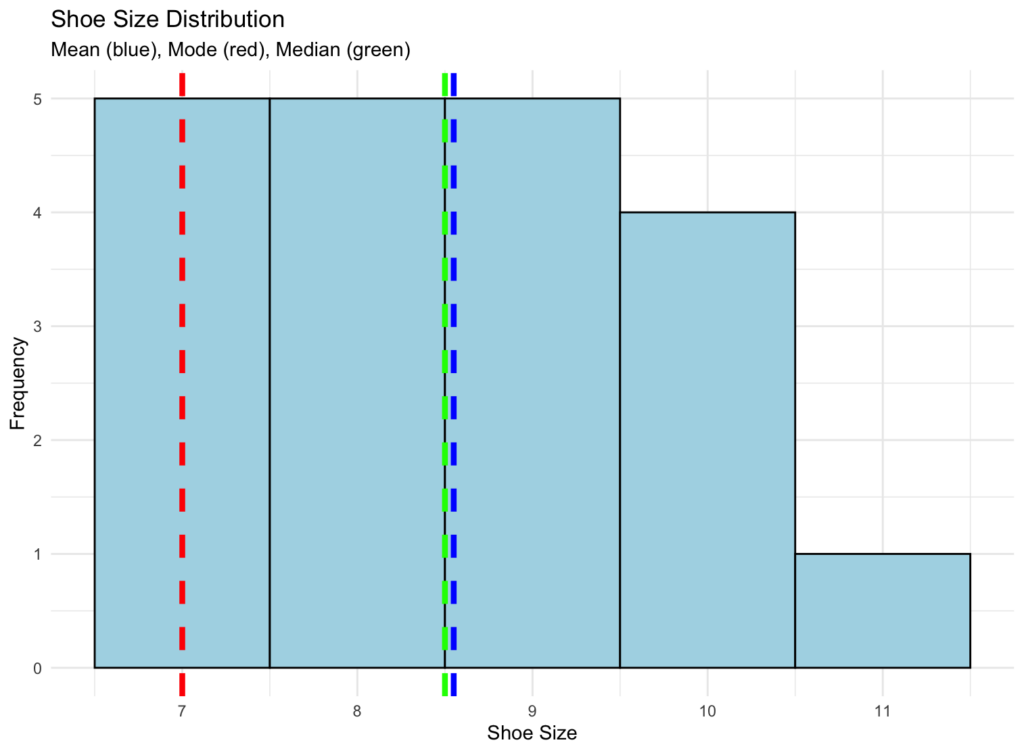 Visualization of mean, mode, and median on a histogram
This visualization helps you see how these three measures relate to your data distribution. The mode appears at the peak (most frequent value), while the mean and median show different aspects of the data's center.
Relationship Between Mean, Median, and Mode
The relationship between mean, median, and mode reveals important information about your data's distribution and skewness.
In Symmetric (Normal) Distributions
When data is perfectly symmetric and normally distributed (bell-shaped curve):
All three measures converge at the center of the distribution. This is the ideal scenario for most statistical analyses.
Example: Heights of adult males often follow a normal distribution where the average height (mean), middle height (median), and most common height (mode) are all approximately the same.
In Right-Skewed (Positively Skewed) Distributions
When data has a long tail to the right (common with income, house prices):
The mean is pulled toward the tail by extreme high values, while the median remains in the middle, and the mode stays at the peak.
Example: Household income distribution
- Mode: $45,000 (most common income)
- Median: $65,000 (middle value)
- Mean: $85,000 (pulled up by high earners)
In Left-Skewed (Negatively Skewed) Distributions
When data has a long tail to the left:
The mean is pulled toward the tail by extreme low values.
Example: Test scores where most students score high (90s) but a few score very low.
Empirical Relationship Formula
For moderately skewed distributions, there's an approximate relationship:
This empirical relationship can help you estimate one measure when you know the other two, though it's most accurate for unimodal, moderately skewed distributions.
When to Use Mean, Mode, or Median
Each measure of central tendency has specific use cases:
Use Mean when:
- Data is normally distributed (symmetric, bell-shaped)
- You need to consider all values in the dataset
- Performing further statistical calculations (standard deviation, variance)
Use Median when:
- Data has outliers or extreme values
- Data is skewed (not normally distributed)
- Analyzing income, housing prices, or other right-skewed data
- You want a measure resistant to extreme values
Use Mode when:
- Analyzing categorical data (colors, sizes, categories)
- Finding the most common or popular value
- Data has multiple peaks (bimodal or multimodal distributions)
- Working with discrete data (shoe sizes, number of children)
For a deeper understanding of these concepts, read our article on what is a measure of central tendency.
Frequently Asked Questions
Wrapping Up
Calculating mean, mode, and median is fundamental to understanding your data. Each measure provides unique insights into central tendency, and knowing when to use each one is crucial for accurate data analysis.
Whether you calculate these measures by hand for small datasets, use Excel functions for quick analysis, or leverage R for complex statistical work, these tools form the foundation of descriptive statistics. Understanding standard deviation and variance will further enhance your statistical analysis skills.
Practice with different datasets to develop intuition about which measure best represents your data's central tendency.