How To Run Moderation Analysis in R with a Single Moderator

Learning how to run moderation analysis in R is essential for understanding conditional relationships in your research data. This comprehensive guide shows you how to conduct moderation analysis using a single moderating variable, interpret moderating effects, build moderation models, and validate moderation analysis assumptions with step-by-step examples and real data.

Whether you need to understand how a moderating variable changes the relationship between variables, test for moderating effects in your regression models, or learn how to do moderation analysis from data preparation to reporting results, this tutorial covers everything you need. We'll explore moderation analysis in R using the lmtest, car, and interactions packages to perform complete moderator analysis.

This guide teaches you moderation in R fundamentals, how to interpret moderation effects, assess your moderation model fit, and report findings following APA guidelines. You'll master testing moderation analysis assumptions, visualizing interaction effects, and understanding when moderating variables significantly influence your research outcomes.

However, if you are dealing with multiple moderators, check our comprehensive guide on How To Run Multiple Moderation Analyses in R like a pro.

What is Moderation Analysis?

Moderation analysis is an analytical method frequently utilized in statistical research to examine the conditional effects of an independent variable on a dependent variable. In simpler terms, it assesses how a third variable, known as a moderator, alters the relationship between the cause (independent variable) and the outcome (dependent variable).

In the language of statistics, this relationship can be described using a moderated multiple regression equation:

Y = \beta_{0} + \beta_{1}X + \beta_{2}Z + \beta_{3}XZ + \epsilon

Where:

Y represents the dependent variable
X is the independent variable
Z symbolizes the moderator variable
β0, β1, β2, and β3 denote the coefficients representing the intercept, the effect of the independent variable, the effect of the moderator, and the interaction effect between the independent variable and the moderator respectively
ε stands for the error term

In moderation analysis, the key component is the interaction term (β3*XZ). If the coefficient β3 is statistically significant (p-value <0.05), it indicates the presence of a moderation effect.

The value of moderation analysis lies in its ability to reveal conditional relationships. Instead of asking "Does X affect Y?", we ask "Does the X→Y relationship depend on Z?" This helps us understand under what conditions or for whom effects occur.

Assumptions of Moderation Analysis

Several assumptions need to be met when conducting moderation analysis. These assumptions are similar to those for multiple linear regression, given that moderation analysis typically involves multiple regression where an interaction term is included. Here are the main assumptions:

Linearity: The relationship between each predictor (independent variable and moderator) and the outcome (dependent variable) is linear. This assumption can be checked visually using scatter plots we will generate and explain in-depth in this article.
Independence of observations: The observations are assumed to be independent of each other. This is more of a study design issue than something that can be tested for. If your data is time series or clustered, this assumption is likely violated.
Homoscedasticity: This refers to the assumption that the variance of errors is constant across all levels of the independent variables. In other words, the spread of residuals should be approximately the same across all predicted values. This can be checked by looking at a plot of residuals versus predicted values.
Normality of residuals: The residuals (errors) are assumed to follow a normal distribution. This can be checked using a Q-Q plot.
No multicollinearity: The independent variable and the moderator should not be highly correlated. High correlation (multicollinearity) can inflate the variance of the regression coefficients and make the estimates very sensitive to minor changes in the model. Variance inflation factor (VIF) is often used to check for multicollinearity.
No influential cases: The analysis should not be overly influenced by any single observation. Cook's distance can be used to check for influential cases that might unduly influence the estimation of the regression coefficients.

Formulate The Moderation Analysis Model

Let's assume that we are searching for the answer to the following research question:

"How does the relationship between coffee consumption (measured by the number of cups consumed) and employee productivity vary by individual tolerance to caffeine?"

Therefore we we can formulate the following hypothesis:

"The level of an individual's caffeine tolerance moderates the relationship between coffee consumption and productivity."

What we are essentially trying to answer with this hypothesis is whether the impact of coffee consumption on productivity is the same for all individuals, or if it changes based on their caffeine tolerance. In other words, we are investigating if the productivity benefits (or drawbacks) of coffee are the same for everyone, or if they differ based on how tolerant a person is to caffeine.

Therefore, our study consists of the following variables: coffee consumption (independent variable), productivity (dependent variable), and caffeine tolerance (the moderator).

The following diagram explains the type of variables in our study and the relationship between them in the context of moderation analysis:

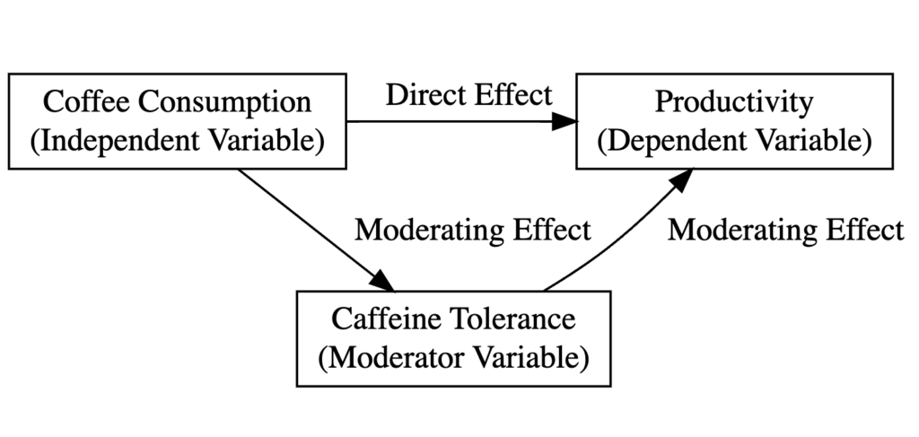Moderation analysis diagram showing coffee consumption as independent variable, productivity as dependent variable, and caffeine tolerance as moderating variable with direct and moderating effect paths Moderation analysis model diagram illustrating the relationship between coffee consumption (X), productivity (Y), and caffeine tolerance (moderator).

Where:

Coffee consumption (Cups) is the independent variable.
Employee productivity (Productivity) is the dependent variable.
Individual tolerance to caffeine (Tolerance) is the moderating variable.
The direct effect shows how coffee consumption impacts productivity overall.
The moderating effect (interaction) shows whether this relationship differs based on caffeine tolerance levels. If significant, it means the coffee-productivity relationship is stronger (or weaker) for people with high vs. low caffeine tolerance.

How To Run Moderation Analysis in R

Now that we've covered enough theoretical ground, it is time to get busy learning how to run moderation analysis in R. We hope that you already have R/R Studio up and running, but if not, here is a quick guide on how to install R and R Studio on your computer.

We will stick with the "coffee" example mentioned earlier for this lesson. Remember, we hypothesized that an individual's caffeine tolerance level moderates the relationship between coffee consumption and productivity.

Step 1: Install and Load Required Packages in R

R offers many packages that help with moderation analysis. In our case, we will use four packages, respectively: lmtest, car, interactions, and ggplots2. Here is a description of each package and its intended purpose:

lmtest: The lmtest package provides tools for diagnostic checking in linear regression models, which are essential for ensuring that our model satisfies key assumptions. This package can perform Wald, F, and likelihood ratio tests. In the context of moderation analysis, you might use lmtest to check for heteroscedasticity (non-constant variance of errors) among other things.
car: The car (Companion to Applied Regression) package is another tool for regression diagnostics and includes functions for variance inflation factor (VIF) calculations, which can help detect multicollinearity issues (when independent variables are highly correlated with each other). Multicollinearity can cause problems in estimating the regression coefficients and their standard errors.
interactions: The interactions package is used to create visualizations and simple slope analysis of interaction terms in regression models. It can produce various types of plots to help visualize the moderation effect and how the relationship between the independent variable and dependent variable changes at different levels of the moderator.
ggplot2: The ggplot2 is one of the most popular packages for data visualization in R. In moderation analysis, ggplot2 can be used to create scatter plots, line graphs, and other visualizations to help you better understand our data and the relationships between variables. Additionally, it can help in visualizing the moderation effect, i.e., how the effect of an independent variable on a dependent variable changes across levels of the moderator variable.

We can install the packages listed above in one go by copying and pasting the following command in the R console:

install.packages("lmtest")
install.packages("car")
install.packages("interactions")
install.packages("ggplot2")

Once installed, load the packages into the R session:

library(lmtest)
library(car)
library(interactions)
library(ggplot2)

Step 2: Import the Data

To make it easier for you to learn how to run moderation analysis in R, you can download the practice dataset from the sidebar - a dummy dataset of 30 respondents containing scores for the variables in our study: coffee consumption (Cups), caffeine tolerance (Tolerance), and productivity (Productivity).

If your dataset is not too large, you can insert the data manually in R in the form of a data frame as follows:

data <- data.frame(
 Respondent = 1:30,
 Cups = c(2, 4, 1, 3, 2, 3, 1, 2, 2, 4, 2, 3, 1, 3, 3, 2, 2, 4, 1, 3, 2, 3, 1, 2, 2, 4, 2, 3, 1, 3),
 Tolerance = c(7, 5, 6, 7, 8, 6, 7, 7, 6, 8, 7, 7, 6, 7, 8, 6, 7, 5, 6, 7, 8, 6, 7, 7, 6, 8, 7, 7, 6, 7),
 Productivity = c(5, 6, 4, 6, 7, 7, 4, 6, 5, 7, 5, 6, 4, 6, 7, 5, 5, 6, 4, 6, 7, 7, 4, 6, 5, 7, 5, 6, 4, 6)
)

IMPORTANT: This dataset can only be used for educational reasons because it contains random values and may not reflect a real-world scenario. The "Cups" (independent variable) reflects the number of cups of coffee consumed per day, "Tolerance" (moderator variable) is a score out of 10 that reflects how well the individual tolerates caffeine, and "Productivity" (dependent variable) is a score out of 10 indicating the individual's productivity level.

Step 3: Fit the Moderated Multiple Regression Model

To fit a moderated multiple regression model, we will use the lm() function in R. Take note that data is our data frame and Cups, Tolerance, and Productivity are columns in that data frame.

model <- lm(Productivity ~ Cups*Tolerance, data)
summary(model)

This command will output the summary of the model including a detailed analysis of the model fit and the significance of each term in the model as we see in the capture below:

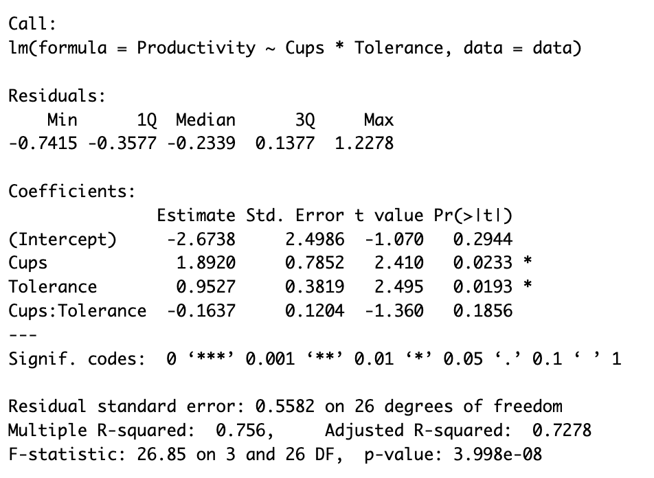R console output showing lm() summary statistics for moderation analysis including coefficients, R-squared values, F-statistic, and interaction term results R output showing moderated multiple regression results with interaction term (Cups:Tolerance) coefficient and significance levels.

Step 4: Interpret the Moderation Effect

The lm() output provides the key information for interpreting moderation. Focus on these coefficients:

Cups: Positive effect (1.8920, p < 0.05) - coffee consumption increases productivity
Tolerance: Positive effect (0.9527, p < 0.05) - higher caffeine tolerance increases productivity
Cups:Tolerance: The interaction term (-0.1637, p > 0.05) - not statistically significant

Since the interaction p-value exceeds 0.05, we conclude there is no significant moderation effect. The relationship between coffee and productivity does not meaningfully depend on caffeine tolerance in this sample.

Model Performance:

R² = 0.756: The model explains 75.6% of productivity variance
Adjusted R² = 0.728: Remains high after adjusting for predictors
F-statistic (p < 0.001): The overall model is statistically significant

Step 5: Visualize the Interaction Effect

We can easily generate a plot to help us visualize the interaction effect using the interact_plot function in R using the following code:

`interactions::interact_plot(model, pred = Cups, modx = Tolerance)`

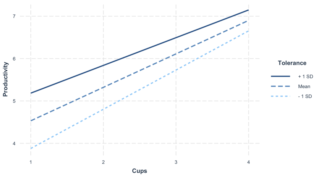Interaction plot showing three lines representing different caffeine tolerance levels and how coffee consumption affects productivity at each tolerance level Interaction plot visualizing the moderating effect of caffeine tolerance on the relationship between coffee consumption and productivity.

This plot shows how the coffee-productivity relationship changes at different tolerance levels. Each line represents a different level of the moderator (low, mean, high tolerance).

Key interpretation:

Non-parallel lines = Moderation exists (the effect of coffee depends on tolerance)
Parallel lines = No moderation (the effect of coffee is the same regardless of tolerance)
Confidence bands show the uncertainty around each slope

Step 6: Assess Model Assumptions and Diagnostics

Before trusting our results, we must verify the regression assumptions: linearity, independence, homoscedasticity, normality, and absence of multicollinearity. We'll also check for outliers and influential observations that could distort our findings.

1. Linearity & Additivity

Plot residuals against fitted values. Random scatter around zero indicates linearity is met.

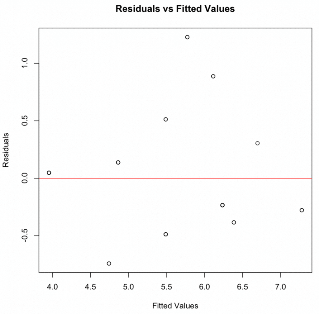Residuals vs fitted values diagnostic plot showing randomly scattered points around horizontal zero line testing linearity assumption in moderation analysis Residuals vs. fitted values plot demonstrating linearity assumption is met with random scatter pattern.

2. Independence of Residuals

The Durbin-Watson test detects autocorrelation in residuals:

`print(dwtest(model))`

Durbin-Watson = 1.9833 (close to 2), p-value = 0.5468 → No autocorrelation. Independence assumption met.

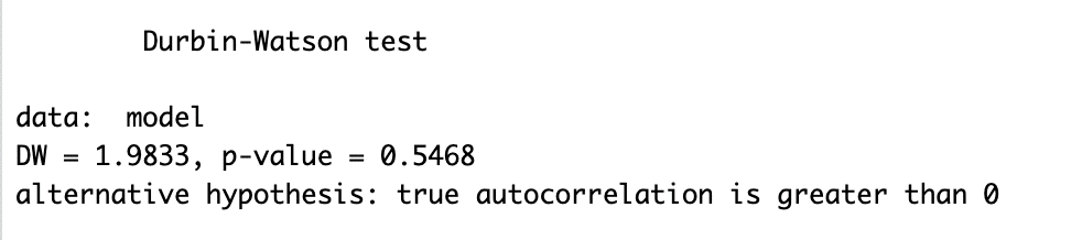R console output displaying Durbin-Watson test results with DW statistic of 1.9833 and p-value of 0.5468 indicating no autocorrelation Durbin-Watson test output showing DW = 1.9833, confirming independence of residuals assumption.

3. Homoscedasticity

Check for equal variance of residuals across fitted values:

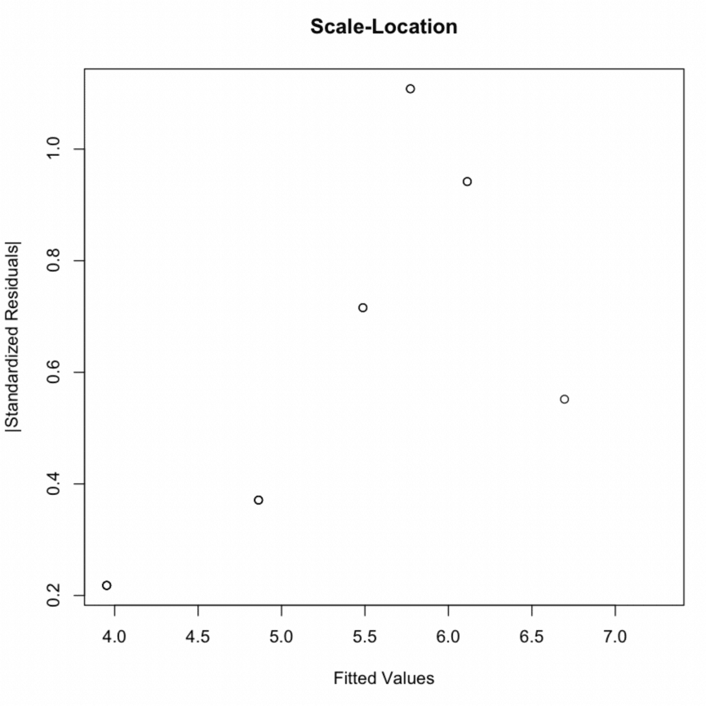Scale-Location plot showing square root of standardized residuals against fitted values testing homoscedasticity assumption with relatively flat red line Scale-Location diagnostic plot demonstrating homoscedasticity with constant variance across fitted values.

Confirm with the Breusch-Pagan test:

`print(bptest(model))`

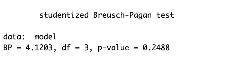R console showing Breusch-Pagan test results with BP statistic of 4.1203 and p-value of 0.2488 confirming homoscedasticity Breusch-Pagan test output with p-value = 0.2488, confirming equal variance assumption is met.

P-value = 0.2488 > 0.05 → Homoscedasticity assumption met.

4. Normality of Residuals

Use a Q-Q plot to check if residuals follow a normal distribution. Points should lie along the diagonal line.

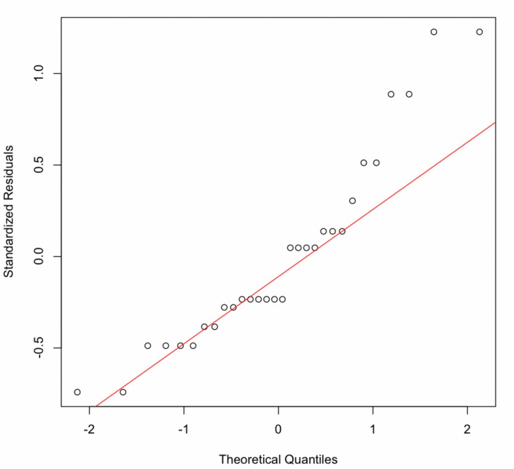Q-Q plot showing theoretical quantiles vs standardized residuals with points partially following diagonal line testing normality assumption Normal Q-Q plot showing residuals partially following the diagonal line with slight deviations at the tails.

The Q-Q plot shows slight deviations. Confirm with the Shapiro-Wilk test:

`shapiro.test(resid(model))`

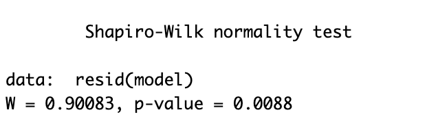R console displaying Shapiro-Wilk normality test results with W statistic of 0.91229 and p-value of 0.008773 for residuals Shapiro-Wilk test output showing p-value = 0.0088, indicating slight departure from perfect normality.

P-value = 0.0088 < 0.05 indicates the residuals are not perfectly normally distributed. However, with small samples (n=30), this test is highly sensitive to minor deviations. The Q-Q plot shows only slight departures, and regression is robust to moderate normality violations due to the Central Limit Theorem.

5. Multicollinearity

Check for multicollinearity using variance inflation factor (VIF). VIF > 10 indicates high multicollinearity.

`print(vif(model))`

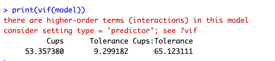R console showing variance inflation factor VIF values with Cups at 53.36, Tolerance at 9.30, and interaction term at 65.12 indicating expected multicollinearity VIF output showing expected high multicollinearity due to interaction term in moderation analysis.

VIF values: Cups = 53.36, Tolerance = 9.30, Cups:Tolerance = 65.12. These high values are expected and acceptable in moderation analysis. Interaction terms are by definition correlated with their component variables. To reduce VIF, center variables before creating the interaction term (subtract the mean from each value).

6. Outliers and Influential Observations

Detect outliers using the Bonferroni outlier test:

`print(outlierTest(model))`

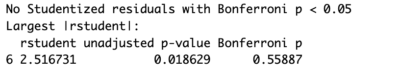R console showing Bonferroni outlier test results with largest studentized residual of 2.516731 at observation 6 and Bonferroni p-value of 0.55887 Bonferroni outlier test output indicating no statistically significant outliers after multiple testing correction.

Observation 6 has the largest residual (2.517), but Bonferroni p-value = 0.559 > 0.05 → No significant outliers detected.

Check influential observations using Cook's distance:

# Influential observations
influence <- influence.measures(model)

# Print Cook's distance values for each observation
print(influence$is.inf)

# Plot Cook's distance
plot(influence$infmat&#91;, "cook.d"],
 main = "Cook's distance plot",
 ylab = "Cook's distance",
 ylim = c(0, max(1, max(influence$infmat&#91;, "cook.d"]))))

# Add a reference line for Cook's distance = 1
abline(h = 1, col = "red")

Cook's distance values above 1 indicate highly influential observations.

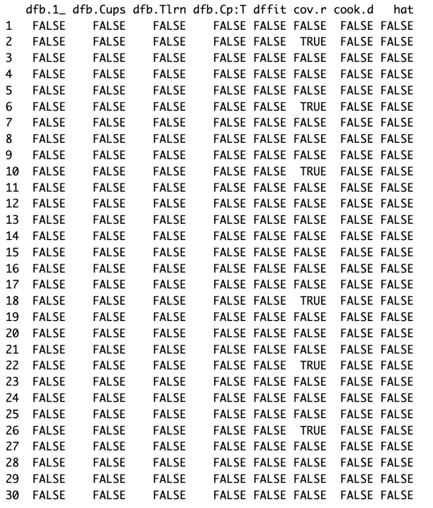Cook's distance values showing no influential observations in moderation analysis in R Cook's distance influence measures for moderation analysis in R.

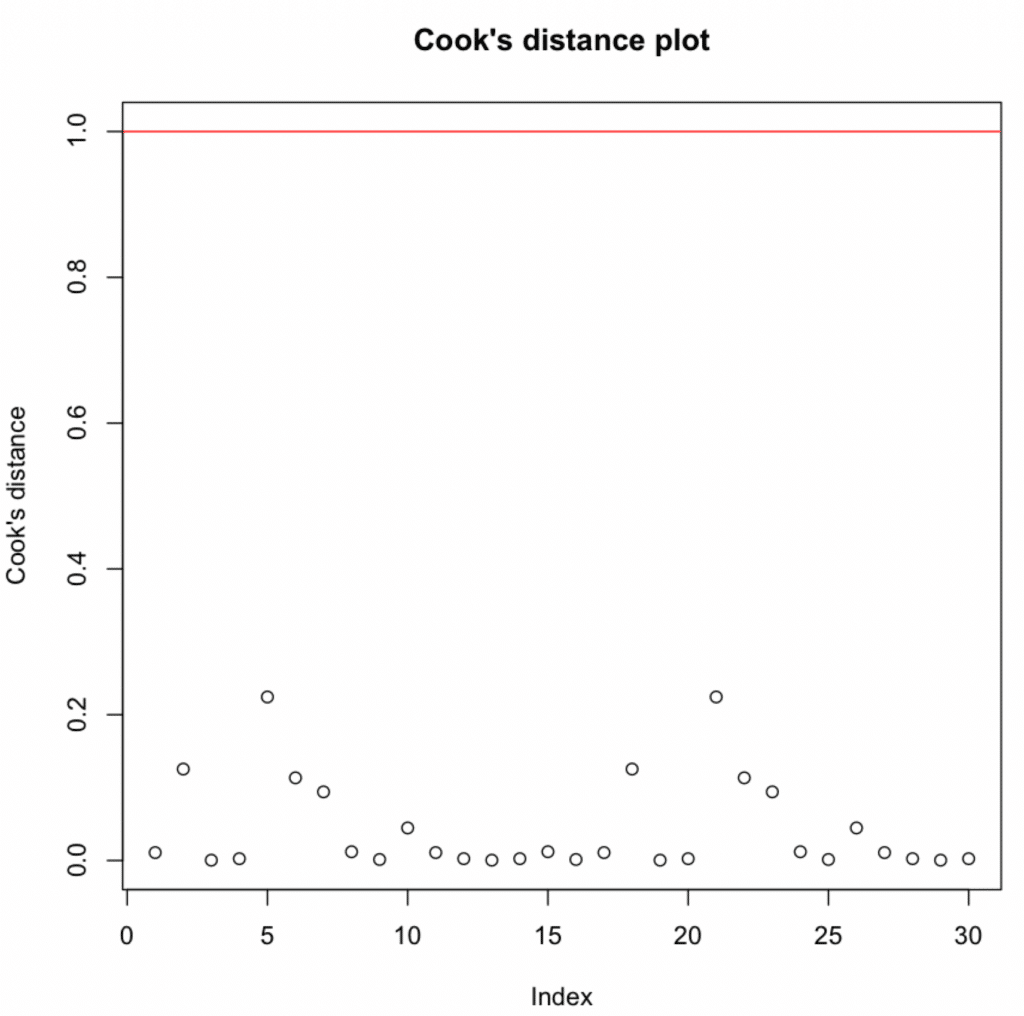Cook's distance plot for moderation analysis in R showing no influential points Cook's distance plot showing all observations below the threshold of 1.

All values are below 1 → No influential observations detected.

Export diagnostic plots to PDF:

# Fit the model
model <- lm(Productivity ~ Cups*Tolerance, data = data)

# Diagnostic Plots
par(mfrow = c(2, 2), oma = c(0, 0, 2, 0))
plot(model, las = 1)
mtext("Diagnostic Plots", outer = TRUE, line = -1, cex = 1.5)

# Save the plots as a PDF file
pdf("Diagnostic_Plots.pdf")
par(mfrow = c(2, 2), oma = c(0, 0, 2, 0))
plot(model, las = 1)
mtext("Diagnostic Plots", outer = TRUE, line = -1, cex = 1.5)
dev.off()

The above script fits the model, creates four relevant diagnostic plots, and then saves these plots as a PDF file named "Diagnostic_Plots.pdf". These diagnostic plots help us to check the assumptions of linearity, independence, homoscedasticity, and absence of influential observations, respectively.

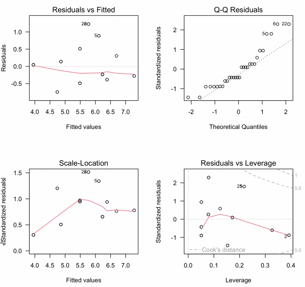Four-panel diagnostic plot showing residuals vs fitted, Q-Q plot, scale-location plot, and residuals vs leverage for comprehensive moderation analysis assumption testing Comprehensive four-panel diagnostic plot for moderation analysis showing all assumption tests in one visualization.

Step 7: Reporting the Results

Finally, it is time to summarize our findings and report the results of the above moderation analysis we conducted in R as follows:

In our moderation analysis in R, we aimed to investigate the effect of caffeine intake (measured by the number of cups of coffee consumed) and stress tolerance on productivity while also considering the potential moderating effect of stress tolerance on the relationship between caffeine intake and productivity. This was achieved through a multiple regression model, specified with an interaction term for cups of coffee and stress tolerance.

The fitted model provided valuable insights into the hypothesized relationships. The interaction term (Cups*Tolerance) was not statistically significant (p > 0.05), suggesting no significant moderation effect of caffeine tolerance on the relationship between coffee consumption and productivity in this sample. This implies that the effect of coffee on productivity does not significantly differ based on an individual's caffeine tolerance level, at least not in this dataset.

Further analysis of model assumptions and diagnostics revealed the model to be a suitable fit for our data:

Linearity & Additivity: The residuals vs fitted values plot indicated that the relationship was linear and additive, with no discernible patterns or deviations from zero mean.
Independence of Residuals: The Durbin-Watson test resulted in a statistic of 1.9833 (p-value = 0.5468), indicating no evidence of autocorrelation in the residuals.
Homoscedasticity: The scale-location plot and the Breusch-Pagan test (p-value = 0.2488) confirmed the assumption of equal variance (homoscedasticity) of residuals.
Normality of residuals: The Shapiro-Wilk test indicated that the residuals did not follow a perfectly normal distribution (p-value = 0.0088 < 0.05). However, given the small sample size (n=30), this test is highly sensitive to minor deviations, and the visual Q-Q plot showed only slight departures from normality. With larger samples, regression models are robust to moderate violations of normality due to the Central Limit Theorem.
Multicollinearity: Variance inflation factors (VIFs) for the predictors were above the typical threshold of 5, indicating the presence of multicollinearity. However, considering that this was expected due to the inclusion of interaction terms, this does not invalidate our model.
Outliers and influential observations: The Bonferroni outlier test did not detect any significant outliers. The Cook's distance values were all below the threshold of 1, suggesting no overly influential points.

In conclusion, our moderation analysis in R did not find a statistically significant moderation effect of caffeine tolerance on the relationship between coffee consumption and productivity. While the model explained a substantial proportion of variance (R² = 0.756), the interaction term was not significant. This suggests that, in this sample, the effect of coffee on productivity does not significantly vary based on caffeine tolerance levels. These findings highlight the importance of adequate sample size and the need for replication studies to detect moderation effects reliably.

IMPORTANT: Please remember to adjust the interpretation to your actual results and context. This is a generic example and might not align completely with your specific research goals and outcomes.

Frequently Asked Questions

How do I run moderation analysis in R?

To run moderation analysis in R: (1) Install required packages (lmtest, car, interactions, ggplot2), (2) Load your data with independent variable, moderator, and dependent variable, (3) Create interaction term using X*Z syntax, (4) Fit model with lm(Y ~ X*Z, data), (5) Check summary output for interaction effect significance, (6) Visualize with interact_plot(), (7) Test assumptions. The interaction term (X:Z) indicates whether moderation is present.

What is a moderating variable in statistics?

A moderating variable (or moderator) is a third variable that affects the strength or direction of the relationship between an independent variable and dependent variable. For example, if studying the effect of coffee consumption on productivity, caffeine tolerance could be a moderating variable - the effect of coffee might be stronger for people with high tolerance versus low tolerance.

What are the assumptions of moderation analysis?

Moderation analysis assumptions include: (1) Linearity - linear relationship between predictors and outcome, (2) Independence of observations - no autocorrelation, (3) Homoscedasticity - constant variance of residuals, (4) Normality of residuals - errors are normally distributed, (5) No multicollinearity - independent variable and moderator not highly correlated (VIF < 10), (6) No influential cases - no single observation unduly influences results (Cook's distance < 1).

How do I interpret a moderating effect?

To interpret a moderating effect: Look at the interaction term (X:Z) in your regression output. If the p-value is < 0.05, moderation exists - meaning the effect of X on Y changes depending on levels of Z. A positive coefficient means the effect strengthens as Z increases; negative means it weakens. Use interaction plots to visualize how the X-Y relationship changes at different levels of the moderator.

What is the difference between moderation and mediation?

Moderation examines WHEN or FOR WHOM an effect occurs (moderator changes the strength/direction of X→Y relationship), while mediation examines HOW or WHY an effect occurs (mediator explains the mechanism through which X affects Y). Moderation involves interaction effects (X*Z), while mediation involves indirect effects (X→M→Y path). Both answer different research questions about variable relationships.

How do I test moderation analysis assumptions in R?

Test moderation assumptions in R using: (1) Linearity: plot(model) residuals vs fitted, (2) Independence: dwtest(model) for Durbin-Watson test, (3) Homoscedasticity: bptest(model) for Breusch-Pagan test, (4) Normality: shapiro.test(resid(model)) and Q-Q plots, (5) Multicollinearity: vif(model) where values > 10 indicate problems, (6) Influential cases: outlierTest(model) and Cook's distance plots. High VIF is expected with interaction terms.

How do I report moderation analysis results?

Report moderation results by stating: (1) The interaction term coefficient and significance (e.g., β = -0.16, p > 0.05), (2) Whether moderation was found (significant interaction = yes), (3) Model fit statistics (R², F-statistic, p-value), (4) Simple slopes at different moderator levels if significant, (5) All assumption test results (Durbin-Watson, Breusch-Pagan, VIF values), (6) Include interaction plot, (7) Interpret practical significance in context of your research question.

What does a significant interaction term mean in moderation analysis?

A significant interaction term (p < 0.05) means moderation exists - the effect of your independent variable on the dependent variable depends on the level of the moderator. For example, if X:Z is significant, it means Z moderates the X→Y relationship. The relationship between X and Y is different at low vs. high levels of Z. This is visualized as non-parallel lines in an interaction plot.

How do I visualize moderation effects in R?

Visualize moderation in R using interact_plot() from the interactions package: interact_plot(model, pred = IndependentVar, modx = Moderator). This creates a plot showing how the relationship between your predictor and outcome changes at different levels of the moderator (typically mean, +1 SD, -1 SD). Non-parallel lines indicate moderation; parallel lines suggest no moderation effect.

What is a moderation model?

A moderation model is a statistical model that tests whether a third variable (moderator) influences the strength or direction of the relationship between an independent and dependent variable. The model equation is: Y = β₀ + β₁X + β₂Z + β₃XZ + ε. The interaction term (β₃XZ) is key - if significant, it indicates moderation. This tests conditional effects rather than direct effects.

Why is my VIF high in moderation analysis?

High VIF (Variance Inflation Factor) values in moderation analysis are expected and normal when you include interaction terms. The interaction term (X*Z) is mathematically correlated with its component variables (X and Z) by definition. VIF > 10 for main effects is typically acceptable in moderation models. To reduce multicollinearity concerns, you can mean-center your variables before creating the interaction term, which often lowers VIF values.

How do I interpret moderating variables?

Interpret moderating variables by examining: (1) Is the interaction significant? If yes, moderation exists, (2) What's the direction of the coefficient? Positive = strengthening effect, negative = weakening effect, (3) Plot simple slopes at different moderator levels (low, mean, high) to see how the X-Y relationship changes, (4) Report effect sizes at specific moderator values, (5) Discuss practical implications - for whom or under what conditions does X most strongly affect Y?

Wrapping It Up

In this comprehensive guide, you've learned how to run moderation analysis in R from start to finish. You now understand what moderating variables are, how to test for moderating effects, build and assess moderation models, and validate all moderation analysis assumptions using diagnostic tests and visualizations.

You've mastered the essential skills for moderation in R: creating interaction terms, interpreting moderation effects, using the lm() function for moderator analysis, and visualizing results with interaction plots. Whether investigating moderating variables in psychological research, business analytics, or social sciences, you can now confidently conduct complete moderation analysis and report findings following best practices.

The moderation model framework you've learned - testing how moderating variables influence relationships between predictors and outcomes - is fundamental to advanced statistical research. By understanding moderation analysis assumptions, properly interpreting moderating effects, and recognizing when moderation exists in your data, you're equipped to answer sophisticated "for whom" and "under what conditions" research questions.

Remember, every dataset and research question is unique, so adapt these moderation analysis techniques to fit your specific needs. Moderation in R is just one powerful analytical approach - combine it with other methods to reveal the complete story in your data.

If you found this moderation analysis guide informative and want to explore related techniques, check out our article on How To Run Mediation Analysis in R. Mediation analysis helps you understand the 'how' and 'why' of relationships, while moderation analysis reveals the 'when' and 'for whom' - together, they provide comprehensive insights into variable relationships.

Until then, happy analyzing!