Testing for normality in R is crucial before running parametric statistical analyses like t-tests, ANOVA, or linear regression. These tests assume your data follows a normal distribution, and violating this assumption can lead to invalid conclusions.
In this guide, we'll cover visual methods (histograms, QQ plots), statistical tests (Shapiro-Wilk, Kolmogorov-Smirnov, Anderson-Darling), and how to interpret normality test results in R.
What is Normality?
Normality refers to whether data follows a normal distribution. A normal distribution, also called a Gaussian distribution, is a bell-shaped curve characterized by its mean and standard deviation. The mean represents the center of the distribution, while the standard deviation represents the spread of the data around the mean.
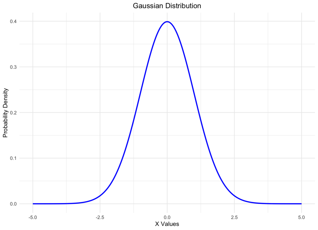
Figure 1: Normal (Gaussian) distribution curve
The normal distribution is important because many parametric statistical tests (t-tests, ANOVA, linear regression) assume that the data being analyzed follows a normal distribution. If your data violates this normality assumption, these statistical tests may produce inaccurate results or invalid conclusions.
Visual Methods to Check Normality in R
Visual methods provide an intuitive way to assess whether your data follows a normal distribution. Here are the two most common visual approaches:
1. Histogram
A histogram is a graphical representation showing the frequency distribution of your data. If data follows a normal distribution, the histogram will display a symmetric, bell-shaped curve.
Here's how to create a histogram in R:
# Create sample data
data <- rnorm(100)

# Create histogram
hist(data, main = "Histogram of Sample Data",
     xlab = "Value", col = "lightblue")
This code generates 100 random numbers from a standard normal distribution (mean = 0, standard deviation = 1) using the rnorm() function and creates a histogram using the hist() function.
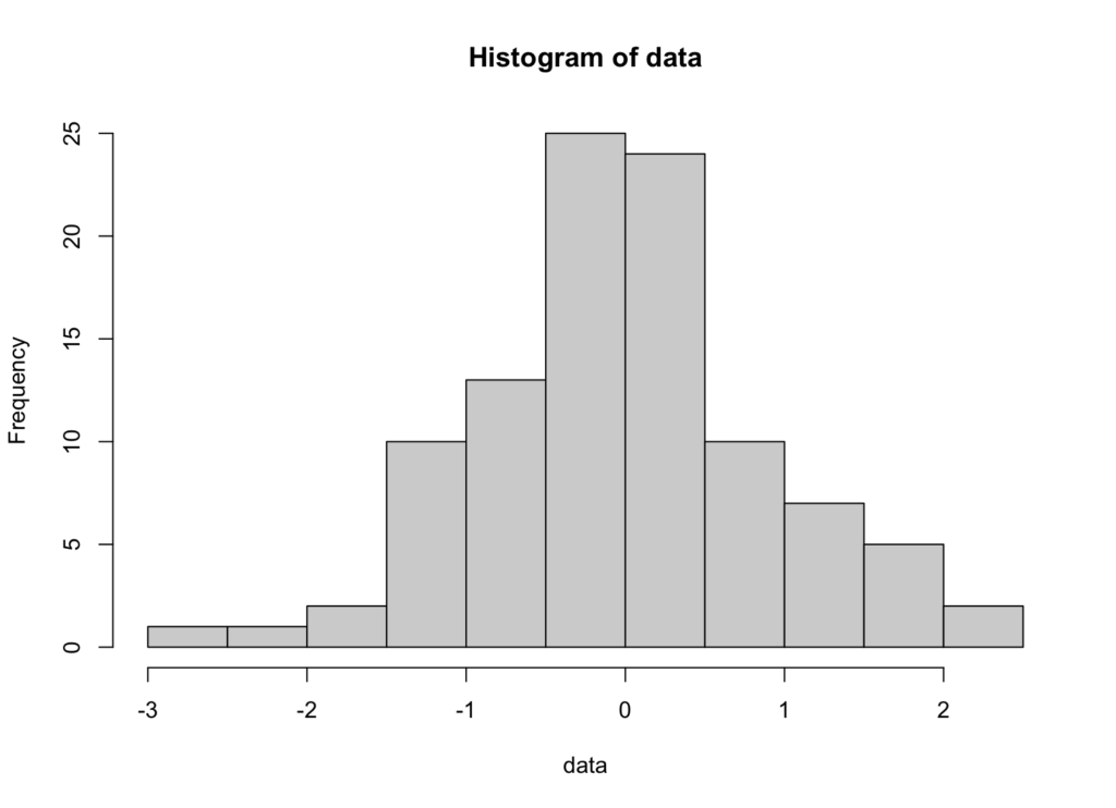
Figure 2: Histogram showing normally distributed data
Interpretation: If the histogram shows a symmetric, bell-shaped curve centered around the mean, your data likely follows a normal distribution. Skewed or multimodal distributions indicate departures from normality.
2. QQ Plot (Quantile-Quantile Plot)
A QQ plot (quantile-quantile plot) compares the quantiles of your data against the quantiles of a theoretical normal distribution. It's one of the most reliable visual methods for assessing normality.
Here's how to create a QQ plot in R:
# Create sample data
data <- rnorm(100)

# Create QQ plot
qqnorm(data, main = "Normal Q-Q Plot")
qqline(data, col = "red")
This code generates 100 random numbers from a standard normal distribution and creates a QQ plot using the qqnorm() function. The qqline() function adds a reference line representing a perfect normal distribution.
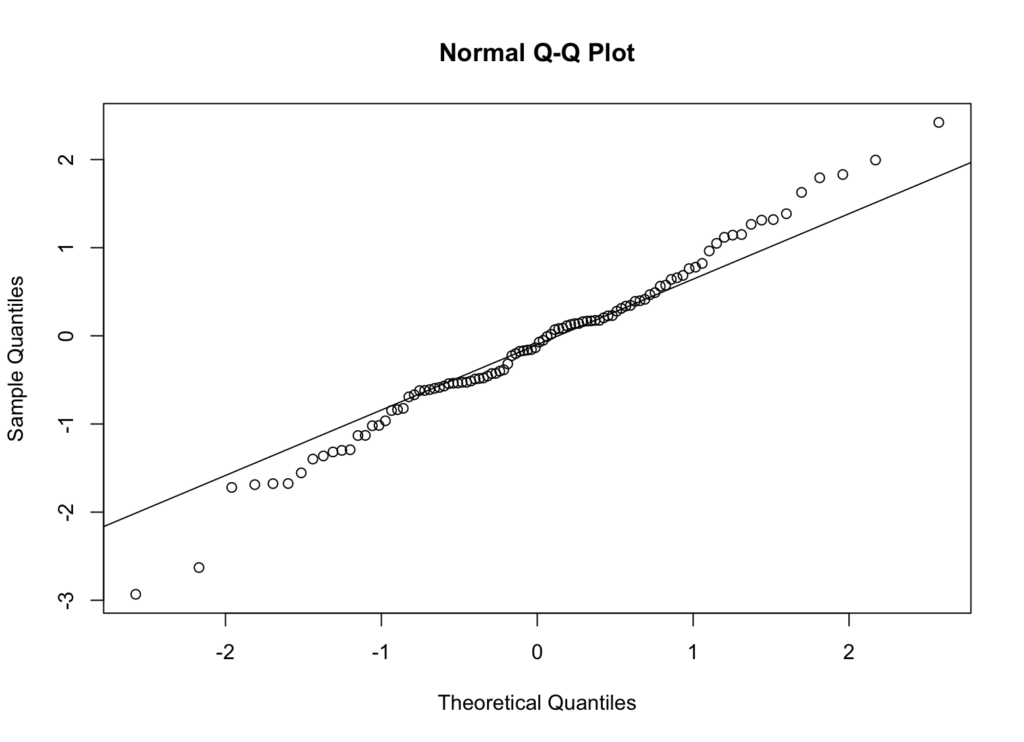
Figure 3: QQ plot for normally distributed data
Interpretation: If your data follows a normal distribution, the points should fall approximately along the reference line. Systematic deviations from the line indicate non-normality:
- Points curving above the line at the ends suggest heavy tails
- Points curving below the line at the ends suggest light tails
- S-shaped patterns indicate skewness
Statistical Tests for Normality in R
While visual methods are useful, statistical tests provide objective, quantitative assessments of normality. Here are the most common normality tests in R:
1. Shapiro-Wilk Test
The Shapiro-Wilk test is one of the most powerful normality tests, especially for small to medium sample sizes (n < 2000).
Hypotheses:
- Null hypothesis (H₀): The data follows a normal distribution
- Alternative hypothesis (H₁): The data does not follow a normal distribution
Here's how to perform the Shapiro-Wilk test in R:
# Create sample data
data <- rnorm(100)

# Perform Shapiro-Wilk test
shapiro.test(data)
This code generates 100 random numbers from a standard normal distribution and performs a Shapiro-Wilk test using the shapiro.test() function.
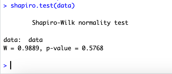
Figure 4: Shapiro-Wilk test results
Interpretation:
- p-value > 0.05: Fail to reject the null hypothesis; data appears normally distributed
- p-value ≤ 0.05: Reject the null hypothesis; data significantly deviates from normality
Note: The Shapiro-Wilk test can be overly sensitive with large sample sizes, detecting trivial departures from normality that have little practical impact.
2. Kolmogorov-Smirnov Test
The Kolmogorov-Smirnov (K-S) test compares your data's cumulative distribution function against a theoretical normal distribution.
# Create sample data
data <- rnorm(100)

# Perform Kolmogorov-Smirnov test
ks.test(data, "pnorm", mean = mean(data), sd = sd(data))
Interpretation: Similar to the Shapiro-Wilk test, a p-value > 0.05 suggests the data follows a normal distribution.
Note: The K-S test is less powerful than the Shapiro-Wilk test for detecting departures from normality, especially in the tails of the distribution.
3. Anderson-Darling Test
The Anderson-Darling test places more weight on the tails of the distribution than the Kolmogorov-Smirnov test, making it more sensitive to deviations in the tails.
# Install and load package if needed
# install.packages("nortest")
library(nortest)

# Create sample data
data <- rnorm(100)

# Perform Anderson-Darling test
ad.test(data)
Interpretation: A p-value > 0.05 indicates the data is consistent with a normal distribution.
Choosing the Right Normality Test
Different normality tests have different strengths and are suited for different situations:
Shapiro-Wilk Test:
- Best for small to medium sample sizes (n < 2000)
- Most powerful normality test
- Can be overly sensitive with large samples
Kolmogorov-Smirnov Test:
- Suitable for any sample size
- General-purpose test
- Less powerful than Shapiro-Wilk
Anderson-Darling Test:
- Good for detecting deviations in distribution tails
- Works with any sample size
- Requires the nortest package
Recommendation: For most applications with sample sizes under 2,000, use the Shapiro-Wilk test combined with QQ plots for visual confirmation.
Frequently Asked Questions
Wrapping Up
Testing for normality in R is a fundamental skill for data analysts and statisticians. This guide covered both visual methods (histograms and QQ plots) and statistical tests (Shapiro-Wilk, Kolmogorov-Smirnov, and Anderson-Darling) to assess whether your data follows a normal distribution.
Remember to use a combination of approaches: start with visual inspection using histograms and QQ plots, then confirm with statistical tests like the Shapiro-Wilk test. Understanding normality is essential before conducting parametric statistical analyses, as violations of the normality assumption can lead to incorrect conclusions.
For most applications with sample sizes under 2,000, the Shapiro-Wilk test combined with QQ plot visualization provides the most reliable assessment of normality in R.
References
Shapiro, S. S., & Wilk, M. B. (1965). An analysis of variance test for normality (complete samples). Biometrika, 52(3-4), 591-611.
Razali, N. M., & Wah, Y. B. (2011). Power comparisons of Shapiro-Wilk, Kolmogorov-Smirnov, Lilliefors and Anderson-Darling tests. Journal of Statistical Modeling and Analytics, 2(1), 21-33.