Homoscedasticity is a fundamental assumption in linear regression and statistical modeling. Understanding what homoscedasticity means - constant variance of residuals - is essential for producing valid, reliable statistical results.
This guide explains the homoscedasticity assumption in statistics, how to recognize violations (heteroscedasticity), and practical solutions. You'll learn the key difference between homoscedasticity vs heteroscedasticity and why violating this assumption leads to unreliable hypothesis tests and confidence intervals in regression analysis.
What is Homoscedasticity Assumption?
Homoscedasticity (pronounced "homo-sked-asticity") describes the constant variance of residuals or errors across all levels of independent variables in a dataset.
Definition: In a homoscedastic dataset, the spread of data points remains consistent regardless of the predictor variable values. The variance doesn't change as the independent variable changes.
Example: In a classroom quiz, if score variability is similar for all ability levels, that's homoscedasticity. All students show similar score spread regardless of their skill.
Heteroscedasticity (the opposite) occurs when variance changes across independent variable levels. In the quiz example, variance might be higher for advanced students and lower for beginners - the spread is not constant.
Homoscedasticity and Linear Regression
Homoscedasticity is a critical assumption in linear regression for several reasons:
-
Efficiency of estimators: When homoscedasticity holds, ordinary least squares (OLS) provides the best linear unbiased estimator (BLUE) with the smallest variance. Heteroscedasticity makes OLS estimators inefficient.
-
Validity of hypothesis tests: Hypothesis tests (t-tests, F-tests) assume homoscedasticity. Violations lead to unreliable test statistics and p-values, causing incorrect conclusions about coefficient significance.
-
Confidence intervals: Homoscedastic data produces accurate confidence intervals. Heteroscedasticity creates intervals that are too wide or narrow, leading to incorrect inferences.
-
Predictive accuracy: With constant variance, model predictions are consistently reliable across all predictor levels. Heteroscedasticity compromises predictive accuracy as residual variability changes.
Recognizing Homoscedasticity (and Heteroscedasticity)
Now that we've covered what homoscedasticity is and why it's important let's discuss how to recognize it in your data. There are a few different ways to check for homoscedasticity, including graphical methods and statistical tests.
Graphical Methods
Create a scatterplot of residuals against fitted values. In homoscedastic data, points should be evenly dispersed with no noticeable patterns or clusters.
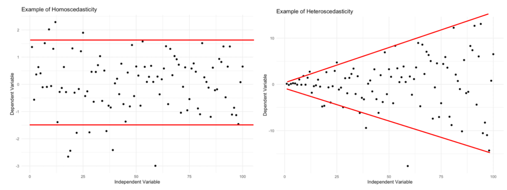
Figure 1: Homoscedasticity vs. heteroscedasticity: constant variance (left) versus changing variance (right).
Statistical Tests
If you prefer a more formal approach, there are several statistical tests available to check for homoscedasticity. Some popular tests include:
-
Bartlett's Test: Checks for equal variances in multiple groups. Significant results indicate heteroscedasticity.
-
Levene's Test: Similar to Bartlett's Test, Levene's Test checks for equal variances across groups. Less sensitive to non-normality, making it more robust.
-
Breusch-Pagan Test: Used in regression analysis. Tests whether squared residuals relate to independent variables. Significant results indicate heteroscedasticity.
-
White Test: More general test for heteroscedasticity in regression. Examines whether squared residuals relate to linear or quadratic combinations of independent variables.
For practical implementation, see our guide on how to test homoscedasticity in R with both graphical and statistical methods (Breusch-Pagan test).
Keep in mind that no single test is perfect, and each has its limitations. In some cases, it might be helpful to use multiple tests or combine them with graphical methods to get a more accurate assessment of homoscedasticity.
Addressing Heteroscedasticity
If you find that your data is heteroscedastic, there are several strategies to address this issue:
-
Transformation: Transform variables (logarithm, square root, reciprocal) to stabilize variance. Note that transformation changes result interpretation.
-
Weighted Regression: Give more weight to observations with smaller variances, less weight to larger variances. Stabilizes variance across predictor ranges.
-
Robust Regression: Uses methods less sensitive to outliers and assumption violations. Provides more accurate estimates with heteroscedastic data.
-
Bootstrapping: Resampling technique that provides accurate population parameter estimates even with heteroscedasticity.
Homoscedasticity vs. Heteroscedasticity: Key Differences
| Aspect | Homoscedasticity | Heteroscedasticity |
|---|---|---|
| Variance | Constant across all predictor levels | Changes across predictor levels |
| Visual pattern | Random scatter, no patterns | Funnel or fan shape |
| OLS efficiency | BLUE (Best Linear Unbiased Estimator) | Inefficient, larger standard errors |
| Hypothesis tests | Valid p-values and confidence intervals | Unreliable p-values, incorrect inferences |
| Impact | Trustworthy results | Biased standard errors, misleading tests |
Table 1: Comparison of homoscedasticity tests
Frequently Asked Questions
Wrapping Up
Homoscedasticity - constant variance of residuals - is a critical assumption in linear regression and many statistical tests. Violating this assumption leads to unreliable standard errors, invalid hypothesis tests, and incorrect confidence intervals.
Key points:
- What is homoscedasticity: Constant variance across all predictor levels
- How to check: Visual plots (residual scatter) and statistical tests (Breusch-Pagan, Levene's, White)
- Solutions: Data transformation, weighted regression, robust methods, bootstrapping
- Impact: Ensures valid, trustworthy statistical results
For hands-on implementation, see how to test homoscedasticity in R with practical examples.
References
Breusch, T. S., & Pagan, A. R. (1979). A simple test for heteroscedasticity and random coefficient variation. Econometrica, 47(5), 1287-1294.
Levene, H. (1960). Robust tests for equality of variances. In I. Olkin (Ed.), Contributions to Probability and Statistics (pp. 278-292). Stanford University Press.
White, H. (1980). A heteroskedasticity-consistent covariance matrix estimator and a direct test for heteroskedasticity. Econometrica, 48(4), 817-838.