Linear regression SPSS tutorial covering how to run, calculate, and interpret regression analysis in SPSS. This guide demonstrates how to calculate a linear regression in SPSS using step-by-step instructions with a sample dataset.
You'll learn how to run linear regression in SPSS, interpret the regression equation SPSS output, and understand key statistics including R Square, ANOVA, and coefficients. This tutorial focuses on simple linear regression SPSS analysis - the foundational regression analysis SPSS technique for examining relationships between two variables.
What is Linear Regression Analysis
Linear regression is a fundamental statistical method for examining the relationship between variables. It uses a regression line (also called the least squares line) to model how one or more independent variables (predictors) influence a dependent variable (outcome).
Linear regression is one of the most widely used predictive modeling techniques in research and data analysis, making it essential for students, researchers, and data scientists.
As the name implies, linear regression uses a line (also called the regression line) to measure the relationship between one or more variables. Think of this relationship as the cause (independent variable) and effect (dependent variable) where linear regression generates a line to show the outcome.
In statistics, the independent variable is often called predictor or explanatory variable. The dependent variable is sometimes referred to as the predicted or outcome variable.
There are two types of linear regression:
- Simple linear regression uses ONE independent variable to predict an outcome
- Multiple linear regression uses two or more independent variables
This tutorial focuses on simple linear regression analysis. In research, the prediction relationship is formulated through a hypothesis - for example, investigating the impact of advertising on revenue.
Import Data In SPSS
As this is a hands-on tutorial on calculating a linear regression analysis in SPSS, we will need some data to generate a regression line.
Download the sample dataset below to follow along with this tutorial.
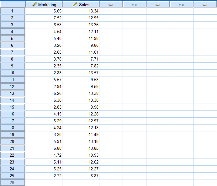
Let’s assume we want to investigate the effect of Advertising on Sales for a given company. Here is what the Excel dataset sample you downloaded above looks like.
Assuming you downloaded the Excel data set above, open SPSS Statistics, and in the top menu, navigate to File → Import Data → Excel.
Browse to the location of the sample Excel file, select it, and click Open. Click OK when prompted to read the Excel file. Once the data set is imported into SPSS, it should look like this:
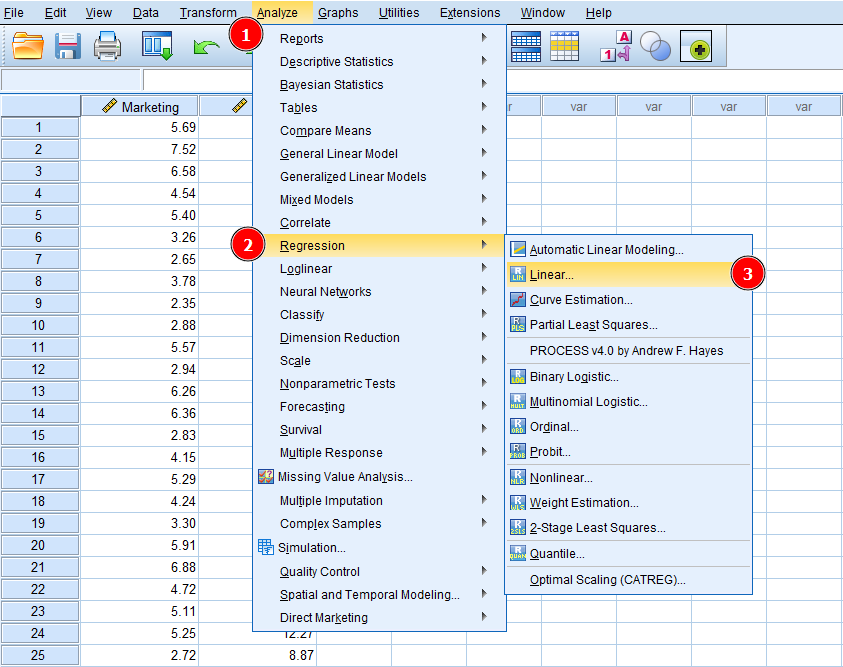
Now, let's find out how to calculate a linear regression in SPSS. On the SPSS top menu navigate to Analyze → Regression → Linear.
 Accessing linear regression in SPSS via Analyze → Regression → Linear.
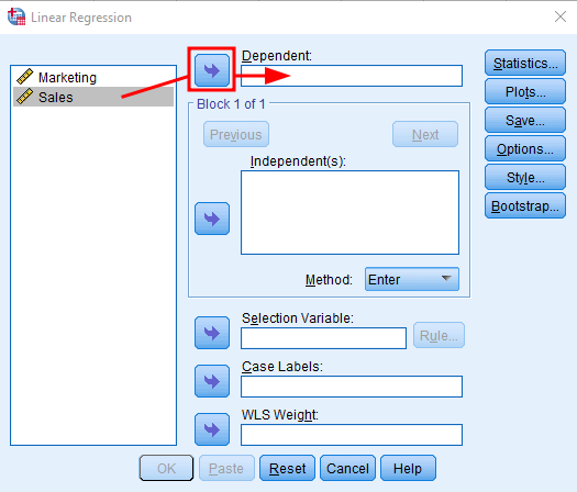
Next, we have to instruct SPSS which is our dependent and dependent variable in the data set.
Remember, in linear regression, we investigate a causal relationship between an independent variable and a dependent variable. In our Excel example, the independent variable is Marketing (cause) and the dependent variable is Sales (effect). In other words, we want to predict if the Sales variable is affected by any changes in the Marketing variable.
In the Linear Regression window, select the Sales variable and click the arrow button next to the Dependent box to add Sales as the dependent variable in the regression analysis.
 Adding the dependent variable (Sales) in SPSS linear regression.
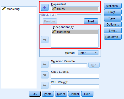
Do the same for the Marketing variable but this time click the arrow next to the Independent box. Your regression analysis window should look like this:
 Adding the independent variable (Marketing) in SPSS linear regression.
We can use other input options to customize the linear regression analysis further, e.g., Method, Statistics, Plots, Style, etc. For now, we will keep things simple and choose the default settings as they are sufficient for this case.
Click OK to start the analysis. And here is how the linear regression analysis results look like in SPSS:
 Complete SPSS linear regression output with all key statistics.
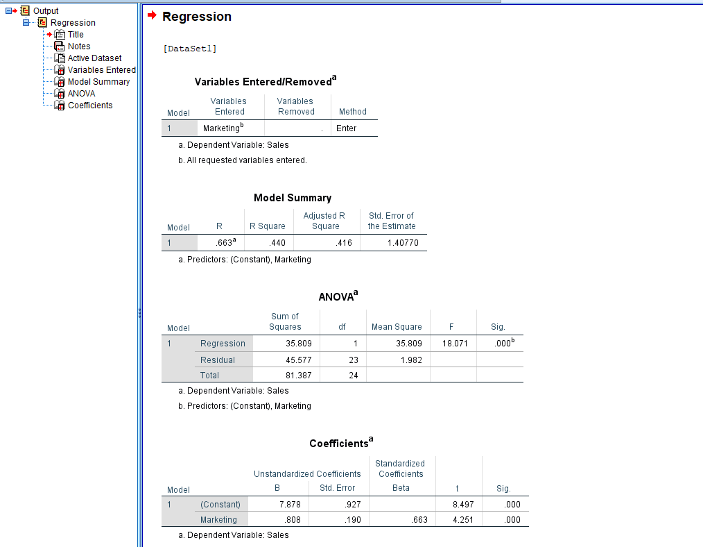
The output shows the independent and dependent variables used in this analysis, the Model Summary, ANOVA, Coefficients, and associated statistics. Let's understand what the regression analysis results tell us.
Understanding Linear Regression Analysis Results
This section explains the meaning of each term and value in the SPSS output, focusing on the most important aspects for your research analysis.
-
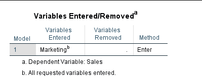
The Variables Entered/Removed table shows a descriptive summary of the linear regression analysis.
-
Model 1 (Enter) simply means that all the requested variables were entered in a single step and are given equal importance. The Enter model is commonly used in regression analysis reason why Model 1 is the default regression model in SPSS.
-
The Variables Entered shows the independent variable (Marketing) used in this analysis. No variables were removed therefore the Variables Removed column is blank.
-
In SPSS, the dependent variable, in our case Sales is specified under the descriptive table.
-
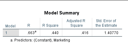
Model Summary table tells us a summary of the results of regression analysis in SPSS.
 SPSS Model Summary table from linear regression output.
- R refers to the correlation variables Correlation is important for regression analysis because we can presume that one variable affects another one if both variables are correlated. If two variables are not correlated, it is probably pointless to look for a cause-and-effect relationship.
Correlation does not warrant a cause and effect relationship but is a necessary condition for a causal relationship to exist.
The R-value ranges from -1 to +1 where -1 is a perfect negative correlation, +1 is a perfect positive correlation and 0 represents no linear correlation between variables.
In our case, R = 0.663 shows the variables Marketing and Sales are correlated.
-
R Square measures the total influence of independent variables on the dependent variable. Note that the R Square value is explained in percentage (%). For instance, in our example, the R Square = 0.440 which means 44% percent of the Sales are influenced by the Marketing strategy of the company.
-
Adjusted R Square is a penalty applied in case your model is non-parsimonious (not simple or efficient). In simple words, if your research conceptual framework contains variables that are unnecessary to predict an outcome, there will be a penalty for it expressed in the Adjusted R Square value.
In our example, the difference between the Adjusted R Square (0.416) and the R Saure (0.440) is 0.024 which is insignificant.
Remember, we should look for simple and not convoluted explanations for the phenomenon under investigation.
- Standard Error of the Estimate refers to how accurate the prediction around the regression line is. If your Standard Error value is between -2 and +2 then the regression line is considered to be closer to the true value.
In our case, the Standard Error of the Estimate = 1.40 which is a good thing.
- ANOVA test is a precursor to linear regression analysis. In other words, it tells us if the linear regression results we got using our sample can be generalized to the population that the sample represents.
Keep in mind that for a linear regression analysis to be valid, the ANOVA result should be significant (p < 0.05). Additionally, regression models should meet key assumptions including homoscedasticity (constant variance), linearity, and normality of residuals.
 SPSS ANOVA table from linear regression output.
- Sum of Squares measures how much the data points in your set deviate from the regression line and helps you understand how well a regression model represents the modeled data.
The rule of thumb for both Regression and Residual Sum of Squares is that the lower the value, the better the data represents your model.
Keep in mind that the Sum of Squares will always be a positive number, with 0 being the lowest value and representing the best model fit.
- DF in ANOVA stands for Degree of Freedom. In simple words, DF shows the number of independent values that were used to calculate the estimate.
Keep in mind that a lower sample size usually means a lower degree of freedom (such as our example). In contrast, a larger sample size allows for a higher degree of freedom which can be useful in rejecting a false null hypothesis and yielding a significant result.
-
Mean Square in ANOVA is used to determine the significance of treatments (factors, respectively the variation in between the sample means. The Mean Square is important in calculating the F ratio.
-
F test in ANOVA is used to find if the means between two populations are significantly different. The F value calculated from the data (F=18.071) is usually referred to as F-statistics and is useful when looking into rejecting a null hypothesis.
-
Sig. stands for Significance. If you don't want to get into the nuts and bolts of the ANOVA test, this is probably the column in the ANOVA result you would like to check first. A Sig. value < 0.05 is considered significant. In our example, Sig. = 0.000 which is less than 0.05, therefore, significant.
Finally, we are ready to move to the regression analysis results table in SPSS.
- In the Coefficients table, only one value is essential for interpretation: the Sig. value respectively the last column - so let's start with it first.
 SPSS Coefficients table from linear regression output.
- Sig. also known as the p-value shows the level of significance that the independent variable has on the dependent variable. Similar to ANOVA, if the Sig. value is < 0.05, there is a significance between the variables in the linear regression.
In our case Sig. = 0.000 shows a strong significance between the independent variable (Marketing) and dependent variable (Sales).
- Unstandardized B (Beta) basically represents the slope of the regression line between independent and dependent variables and tells us for one unit increase in the independent variable how much the dependent variable will increase.
In our case, for every one-unit increase in Marketing, the Sales will increase 0.808. The unit increase can be expressed in, e.g., currency.
The Constant row in the Coefficients table shows the value of the dependent variable when the independent variable = 0.
- Coefficients Std. Error is similar to the standard deviation for a mean.
The larger the Standard Error value is the more spread the data points on the regression line are. The more spread out the data points, the less likely significance will be found between variables.
- Standardized Coefficients Beta value ranges from -1 to +1 with 0 meaning no relationship; 0 to -1 meaning negative relationship and 0 to +1 positive relationship. The closer the Standardized Coefficient Beta value to -1 or +1, the stronger the relationship between variables.
In our case, the Standardized Coefficient Beta = 0.663 shows a positive relationship between the independent variable (Marketing) and the dependent variable (Sales).
- t represents the t-test and is used to calculate the p-value (Sig.). In broader terms, the t-test is used to compare the mean value of two data sets and determine if they originate from the same population.
Frequently Asked Questions
Wrapping Up
As you can see, learning how to calculate a linear regression in SPSS is not difficult. On the other hand, understanding the linear regression output can be a bit challenging, especially if you don't know which values are relevant to your analysis.
The most important thing to keep in mind when assessing the result of your linear regression analysis is to look for statistical significance (Sig. < 0.05).
For advanced regression techniques, explore moderation analysis in SPSS to test interaction effects between variables.