Moderation analysis helps you understand when a relationship between two variables changes. Instead of asking whether X affects Y, moderation analysis asks: "Does the strength of the X→Y relationship depend on a third variable (the moderator)?"
In this guide, you'll learn two practical methods to perform moderation analysis in SPSS: the manual approach with variable standardization and the modern PROCESS Macro method.
What is Moderation Analysis?
Moderation analysis tests whether the relationship between an independent variable (X) and a dependent variable (Y) changes depending on the level of a third variable called the moderator (M).
Think of it this way: The effect of X on Y is not the same for everyone. It depends on M.
Example Research Question: "Does age (M) moderate the relationship between customer relationship quality (X) and consumer loyalty (Y)?"
In this example:
- Independent Variable (X): Customer Relationship Quality
- Moderator Variable (M): Age
- Dependent Variable (Y): Consumer Loyalty
The research question asks: Is the relationship between relationship quality and loyalty stronger or weaker for older vs. younger customers?
Understanding Moderation vs. Mediation
Moderation is fundamentally different from mediation:
Moderation: M changes the strength or direction of the X→Y relationship (interaction effect)
Mediation: M transmits the effect from X to Y (indirect effect)
In moderation, M does not have a causal relationship with X. The moderator is independent of the predictor.
Learn more: Mediators vs. Moderators in Research
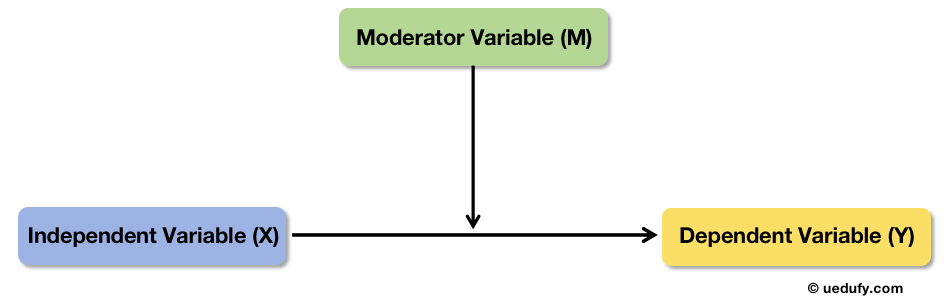 Conceptual diagram of moderation showing how M influences the strength of the X→Y relationship.
The Interaction Term
Moderation is tested using an interaction term (also called product term), calculated as:
Interaction = X × M
When you include this interaction term in a regression model, a significant interaction effect indicates moderation.
Method 1: Manual Moderation Analysis
The manual method requires more steps but helps you understand the underlying mechanics of moderation analysis. This approach involves standardizing variables, creating an interaction term, and running linear regression.
Sample Dataset:
For this tutorial, we'll use a sample dataset with three variables: Relationship, Loyalty, and Age. If you want to follow along, download the sample SPSS data file and import it into SPSS. The dataset should look like this:
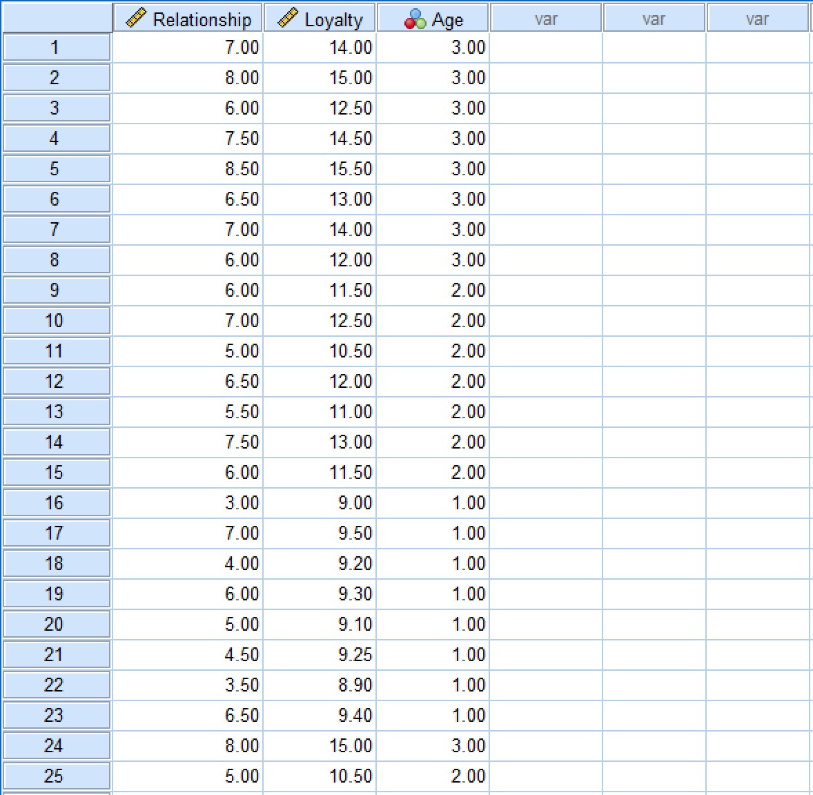 Sample SPSS dataset showing Relationship, Loyalty, and Age variables.
Step 1: Standardize Continuous Variables
Important Note: In this manual method, we'll use Z-score standardization (creating standardized scores with mean = 0 and SD = 1). This is different from mean centering used by PROCESS Macro, which only subtracts the mean (mean = 0 but keeps original SD).
Both approaches reduce multicollinearity between the interaction term and its components. Z-score standardization has the advantage of putting all variables on the same scale, making coefficients directly comparable.
Why Standardize? When you multiply X × M to create the interaction term, the resulting variable is often highly correlated with X and M. Standardization minimizes this issue and makes interpretation easier.
To standardize the variables in our dataset, navigate to Analyze → Descriptive Statistics → Descriptives in the SPSS top menu.
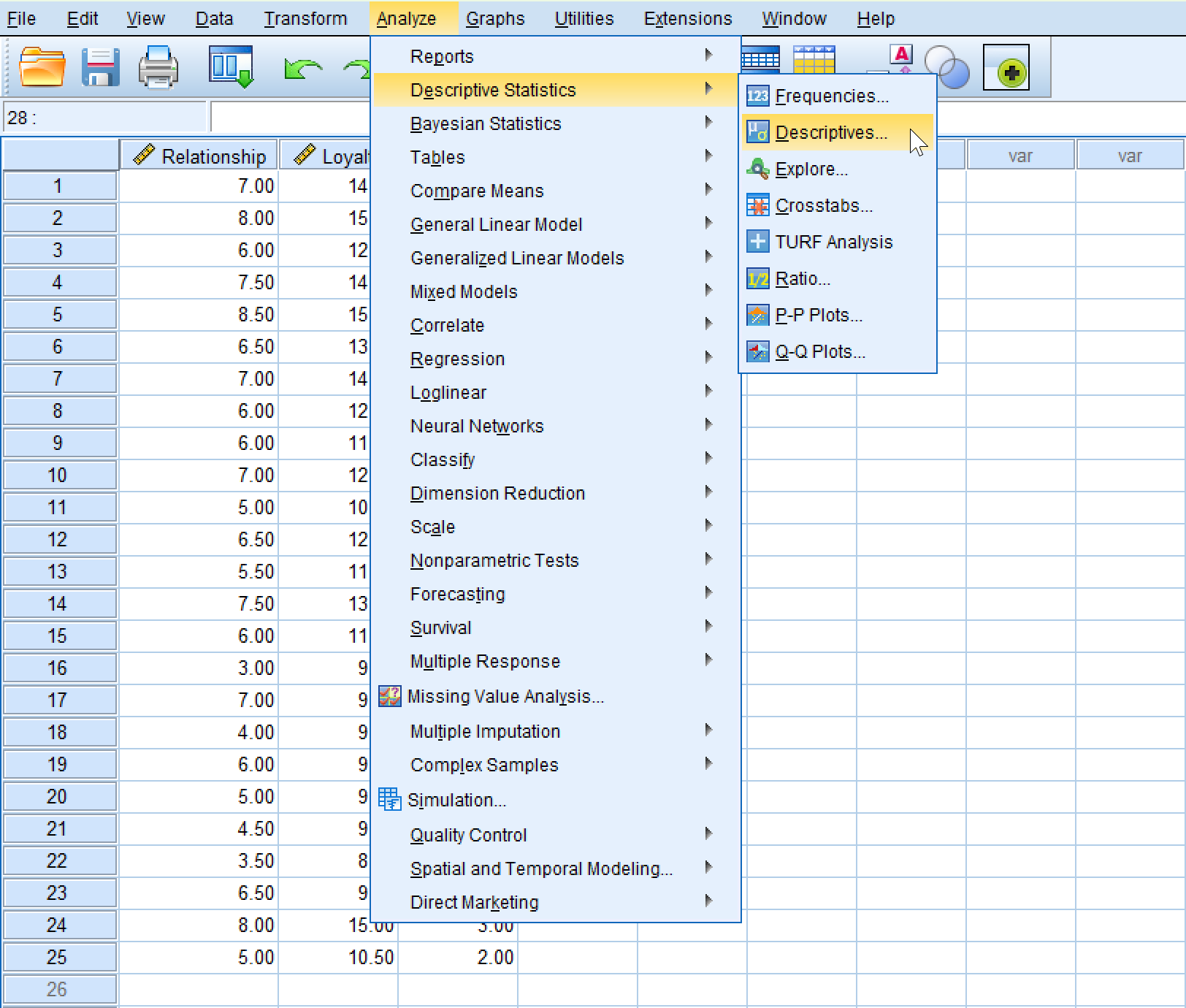 Navigating to Descriptive Statistics in SPSS to center variables.
In the Descriptives window:
- Move Relationship and Age to the Variable(s) box
- Check "Save standardized values as variables"
- Click
OK
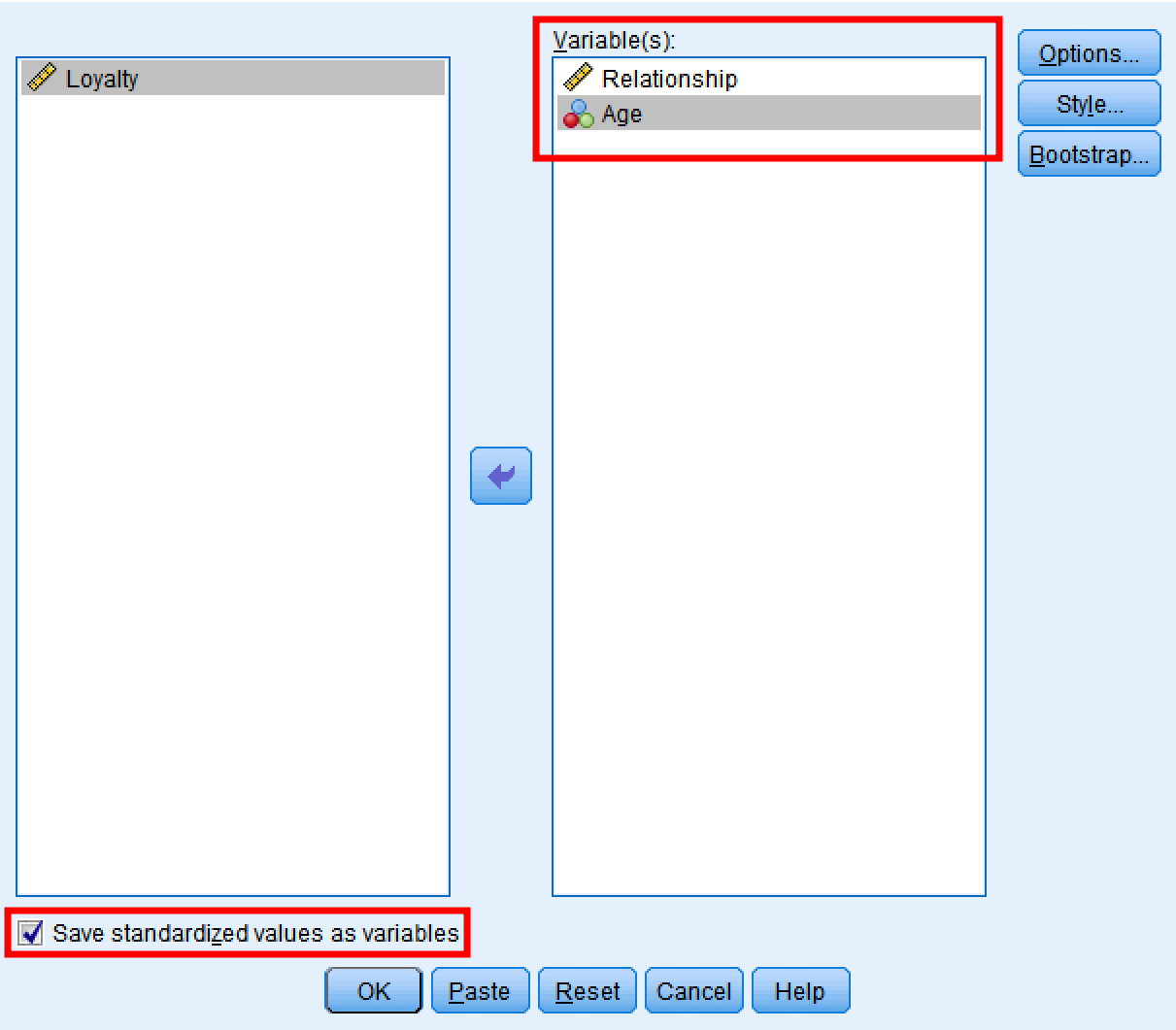 SPSS Descriptives dialog window showing variable selection and standardization options.
SPSS will create new variables with a Z prefix: ZRelationship and ZAge.
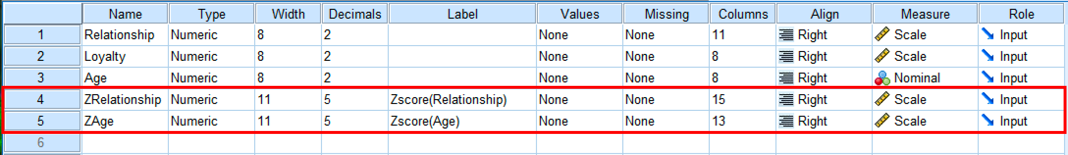 SPSS Data View showing original and standardized variables with Z prefix.
What Standardization Does:
| Before Standardization | After Standardization |
|---|---|
| Original scale (e.g., 1-7) | Z-score scale (mean = 0, SD = 1) |
| Mean varies by variable | Mean = 0 for all variables |
| Different units | Standardized units |
Comparison of original and standardized variables.
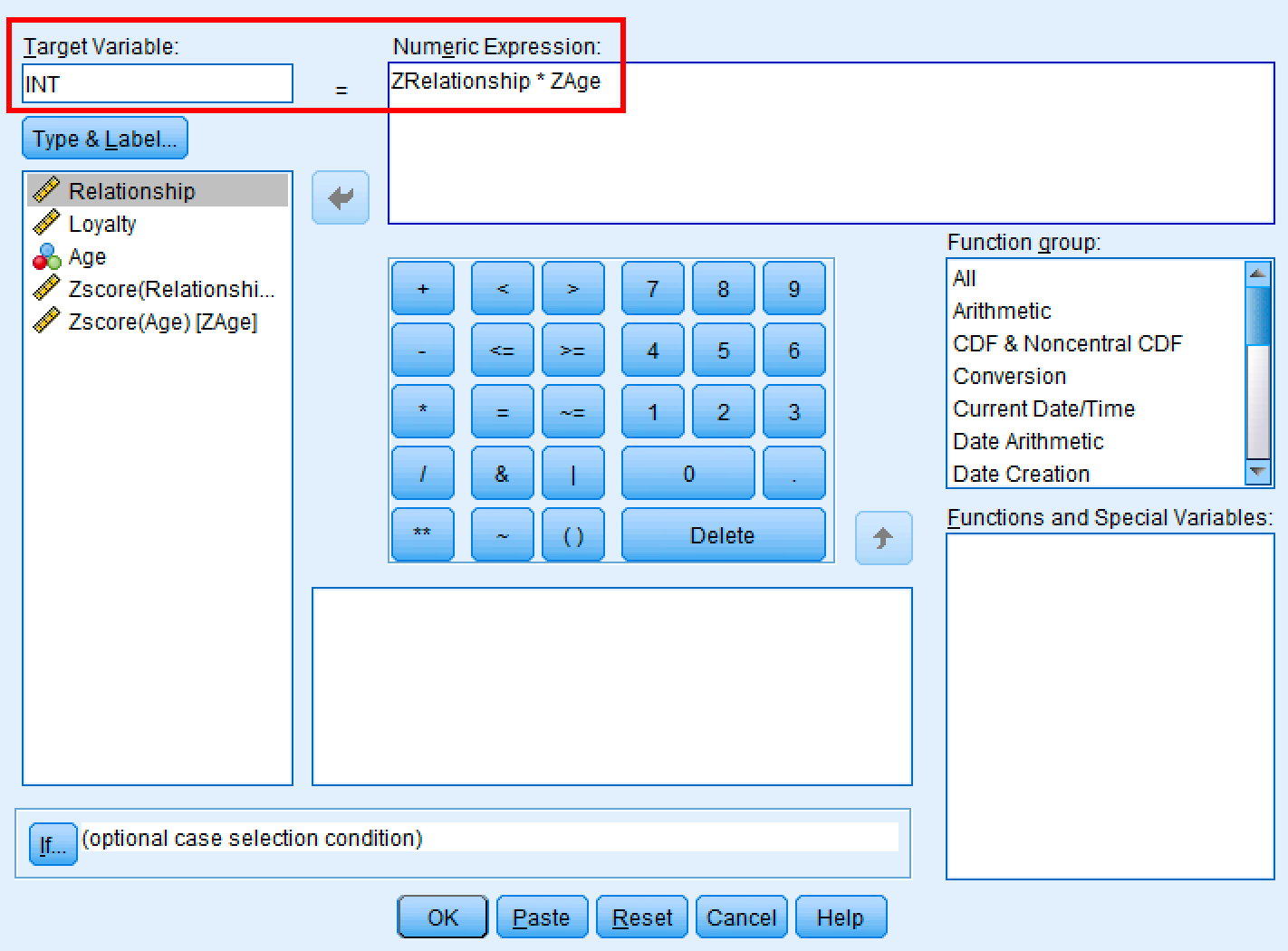
Step 2: Create the Interaction Term
Now create the product term by multiplying the standardized variables.
In SPSS:
- Go to
Transform→Compute Variable - In Target Variable, type:
INT(short for interaction term) - In the Numeric Expression box, type:
ZRelationship * ZAge - Click
OK
 SPSS Compute Variable dialog for creating the interaction term.
SPSS creates a new variable called INT that contains the product of the two standardized variables.
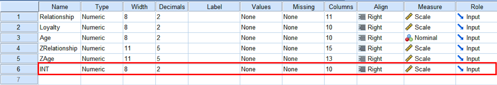 SPSS Data View showing the newly created INT variable.
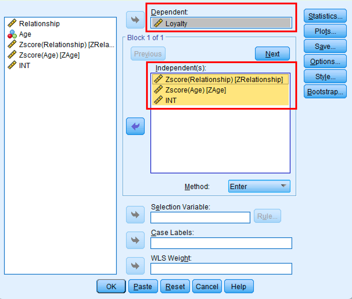
Step 3: Run Linear Regression
Now test whether the interaction term significantly predicts the dependent variable.
In SPSS:
- Go to
Analyze→Regression→Linear - Move Loyalty (Y) to the Dependent box
- Move ZRelationship, ZAge, and INT to the Independent(s) box
- Click
OK
 SPSS Linear Regression dialog for moderation analysis.
Interpret Moderation Analysis in SPSS
The linear regression analysis produces three tables: Model Summary, ANOVA, and Coefficients. To determine if Age moderates the relationship between Relationship and Loyalty, you need to examine the significance value in the Coefficients table.
Step 1: Check the Model Summary Table
First, look at the R Square value in the Model Summary table.
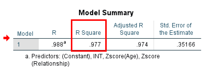 Model Summary table showing R-squared value for the moderation model.
The R Square tells you how much variance in the dependent variable (Loyalty) is explained by your model. In this example, R Square = 0.977, which means the model explains 97.7% of the variation in customer loyalty.
⚠️ Important Note About This Example: This R² value of 0.977 is artificially high because this is simulated data created for teaching purposes. In real research, R² values for moderation models typically range from 0.20 to 0.60. Don't expect to see R² values this high in your actual research. If you do see values above 0.90, it may indicate data issues, overfitting, or that you're working with highly controlled experimental data. This example uses an unrealistic R² to make the statistical patterns clear for learning purposes.
Step 2: Check the ANOVA Table
Next, examine the ANOVA table to test whether your overall regression model is statistically significant.
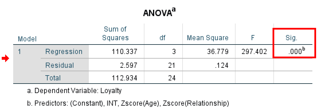 ANOVA table showing overall model significance.
The ANOVA table tests whether your regression model (with all predictors included) explains a statistically significant amount of variance in the outcome variable. Look at the Sig. column:
- If Sig. < 0.05 (often shown as 0.000): Your model is statistically significant. At least one of your predictors (ZRelationship, ZAge, or INT) has a significant effect on Loyalty. This is what you want to see.
- If Sig. > 0.05: Your model is not significant. The predictors do not significantly explain variation in the outcome. This suggests the variables may not have meaningful relationships.
In this example, the ANOVA table shows F = 297.402 with Sig. = .000 (p < 0.001). This highly significant result confirms that the overall model is statistically significant and that the predictors collectively explain a meaningful amount of variance in customer loyalty.
Step 3: Examine the Coefficients Table
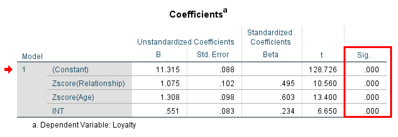
Finally, check the Coefficients table to see if the interaction term (INT) is significant.
 SPSS regression coefficients table showing the interaction effect.
Before interpreting the results, let's understand what each row in the Coefficients table tells you:
| Variable | What It Tells You |
|---|---|
| (Constant) | The baseline value of Loyalty when all predictors are zero |
| Zscore(Relationship) | Main effect of relationship quality on loyalty |
| Zscore(Age) | Main effect of age on loyalty |
| INT | The moderation effect: does the relationship between X and Y change depending on age? |
Understanding the coefficients table in moderation analysis.
Now, look at the row for INT (your interaction term) and check the Sig. column:
- If Sig. < 0.05: The moderator variable (Age) significantly affects the relationship between Relationship and Loyalty. Moderation exists.
- If Sig. > 0.05: Age does not moderate the relationship. No moderation effect.
In this example, the Sig. value for INT is .000 (p < 0.001). This is highly significant, well below the 0.05 threshold. We can confidently conclude that the moderation effect is statistically significant. This means Age does moderate the relationship between Relationship and Loyalty. In other words, the effect of relationship quality on loyalty depends on the customer's age.
Step 4: Interpret the Direction
Once you've confirmed the interaction is significant, you need to understand the direction of the moderation effect. Look at the B (unstandardized coefficient) value in the INT row.
In this example, the B value for INT is 0.551. Since this is a positive coefficient, it tells us the relationship between Relationship and Loyalty becomes stronger as Age increases.
What This Means:
The positive coefficient (B = 0.551) indicates that the effect of relationship quality on loyalty is stronger for older customers than for younger customers. In other words, building strong relationships has a bigger impact on loyalty among older customers compared to younger ones.
Understanding Positive vs. Negative Coefficients:
- Positive coefficient (+): The X→Y relationship becomes stronger as M increases. Higher values of the moderator amplify the effect.
- Negative coefficient (−): The X→Y relationship becomes weaker as M increases. Higher values of the moderator diminish the effect.
In our example, Age enhances the relationship between relationship quality and loyalty.
Method 2: PROCESS Macro (Recommended)
The PROCESS Macro, developed by Andrew Hayes, is the modern standard for moderation analysis. It automatically handles standardization, creates interaction terms, and provides conditional effects at different levels of the moderator.
Installing PROCESS Macro
Before you can use PROCESS, you need to install it in SPSS. The installation takes about 5 minutes.
For detailed installation instructions, see our guide: How to Install PROCESS Macro in SPSS.
Running Moderation with PROCESS
Once PROCESS is installed, you can access it from the SPSS menu.
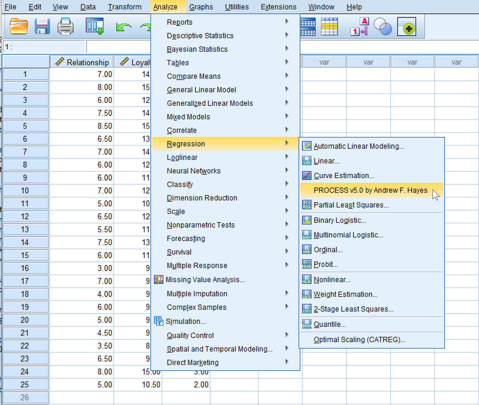 Accessing PROCESS Macro from the SPSS menu: Analyze → Regression → PROCESS.
In SPSS:
- Go to
Analyze→Regression→PROCESS v5.0 by Andrew F. Hayes - Select Model 1 (simple moderation model)
- Move Loyalty to the Y Variable box
- Move Relationship to the X Variable(s) box
- Move Age to the W: Primary Moderator box (not the M: Mediator box)
- Leave M: Mediator(s), Z: Secondary Moderator, and COV: Covariate(s) empty
- Click
Options
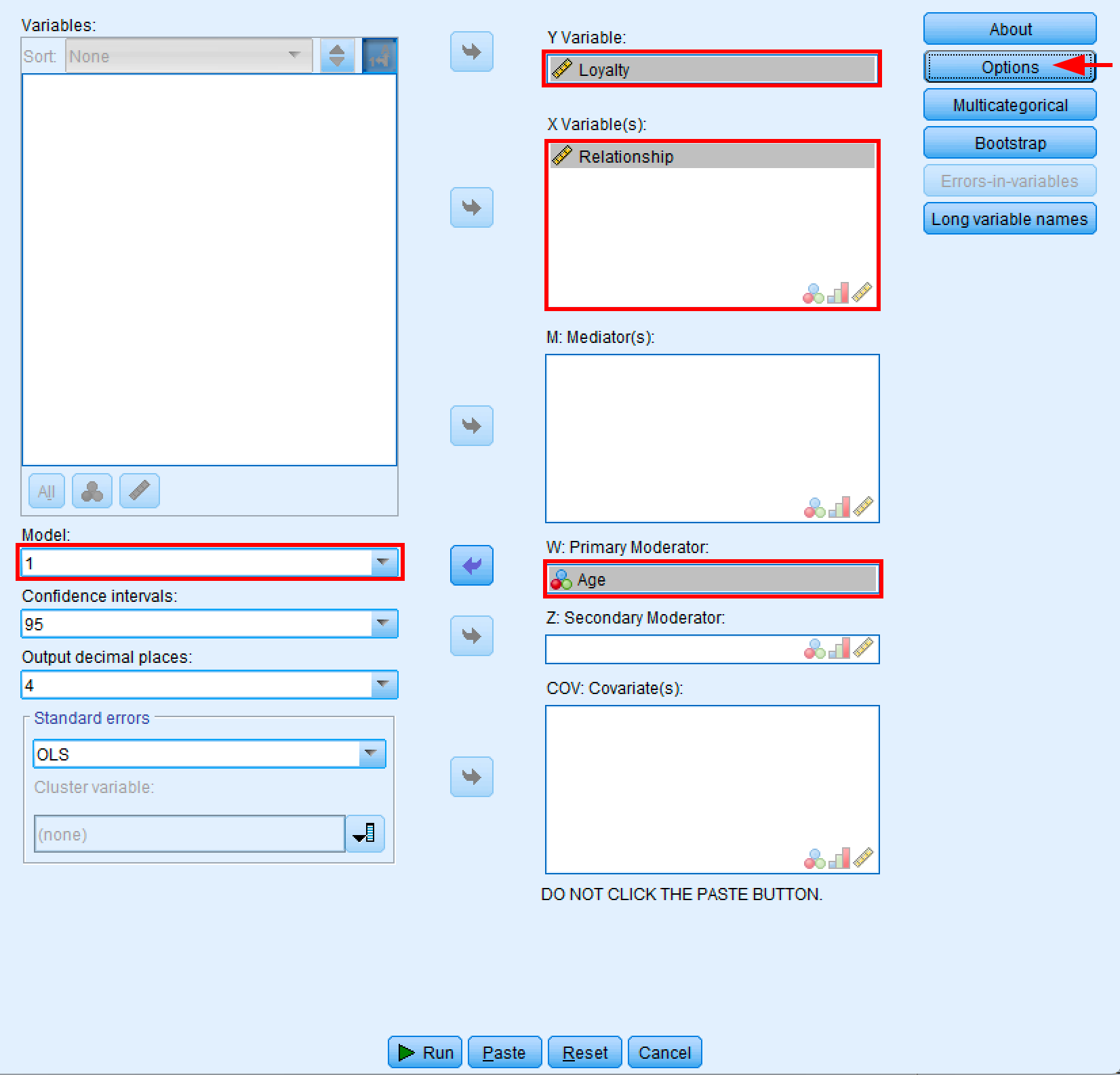 PROCESS Macro dialog box configured for simple moderation analysis using Model 1.
Important: Make sure you place Age in the W: Primary Moderator box, not the M: Mediator(s) box. The M box is for mediation analysis (different models), while the W box is specifically for moderation. If you accidentally put Age in the M box, the moderation options will be grayed out in the Options window.
In the Options window:
- Under "Centering for moderation:" ensure "Mean center components of products" is checked (this automatically centers variables to reduce multicollinearity)
- Keep the default "Continuous and dichotomous components" selected
- Under "Probing moderation:" ensure "Probe interactions" is checked
- Keep the default "Percentiles" selected for moderator values
- Check "Johnson-Neyman technique" to identify regions of significance
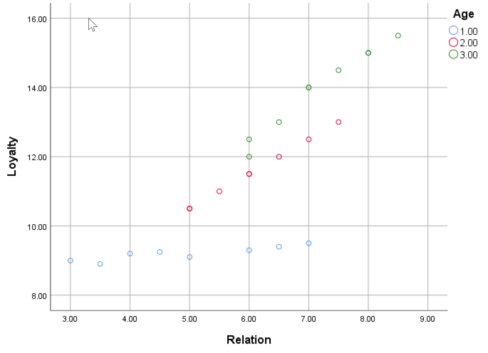
- Under "Visualizing moderation:" check "Generate data to visualize moderation"
- Click
OK
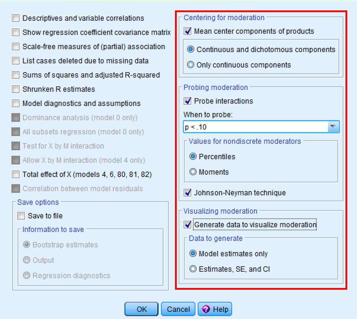 PROCESS options window showing recommended settings for moderation analysis.
Once you've configured the options, click the Run button in the main PROCESS window. PROCESS will execute the analysis and produce comprehensive output in the SPSS Output Viewer.
Understanding PROCESS Output
PROCESS produces the same regression tables you saw in Method 1, but automatically handles all the calculations.
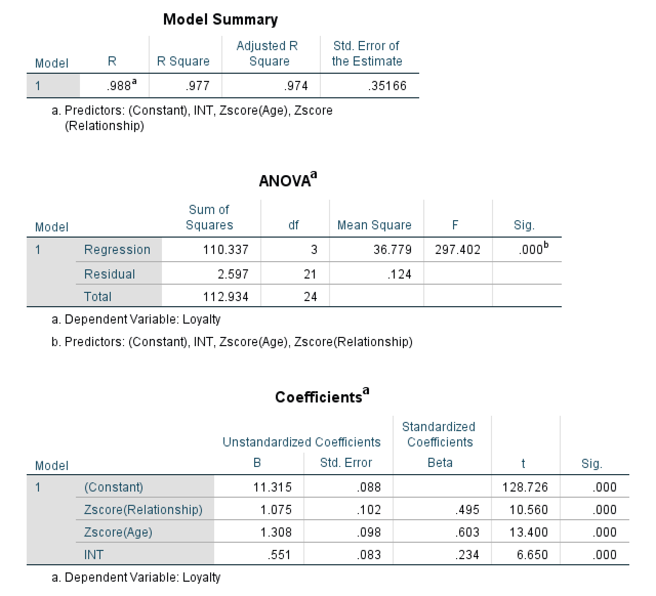 PROCESS output showing Model Summary, ANOVA, and Coefficients tables.
The results are identical to Method 1 (R² = .977, F = 297.402, INT Sig. = .000), confirming the significant moderation effect. For detailed interpretation of the Model Summary, ANOVA, and Coefficients tables, refer to the interpretation section in Method 1.
What PROCESS Adds Beyond Method 1:
The real advantage of PROCESS is the additional output it provides:
- Conditional Effects Table: Shows how the effect of Relationship on Loyalty changes at different Age levels (e.g., low, average, high)
- Johnson-Neyman Output: Identifies the exact Age values where the moderation effect becomes significant or non-significant
- Visualization Data: Pre-computed values ready for plotting the interaction
These features make PROCESS the preferred method for research and publication, as they provide deeper insight into how the moderation works across the full range of moderator values.
Interpreting Simple Slopes (Conditional Effects)
Finding a significant interaction term tells you that moderation exists, but it doesn't tell you how the moderator affects the X→Y relationship. This is where simple slopes analysis becomes critical.
What Are Simple Slopes?
Simple slopes (also called conditional effects) represent the relationship between X and Y at specific values of the moderator. Instead of asking "Does the moderator affect the relationship?" (answered by the interaction term), simple slopes answer: "What is the X→Y relationship at different moderator levels?"
For our example, simple slopes tell us:
- What's the effect of Relationship on Loyalty for younger customers?
- What's the effect of Relationship on Loyalty for average-age customers?
- What's the effect of Relationship on Loyalty for older customers?
PROCESS Conditional Effects Output
When you run PROCESS Model 1 with "Probe interactions" enabled, PROCESS automatically calculates simple slopes at three moderator values:
PROCESS conditional effects output showing the relationship between Relationship Quality and Loyalty at low, mean, and high Age levels.
What each column means:
| Column | Meaning |
|---|---|
| Age | The moderator value (centered). Negative = below mean, 0 = mean, positive = above mean |
| Effect | The slope of Relationship→Loyalty at this Age level (this is your simple slope) |
| se | Standard error of the effect |
| t | T-statistic testing if this simple slope is significantly different from zero |
| p | P-value. If p < .05, the X→Y relationship is significant at this moderator level |
| LLCI, ULCI | 95% confidence interval. If doesn't include zero, effect is significant |
Understanding the PROCESS conditional effects table.
How to Interpret Simple Slopes
Using the values from our analysis, here's how to interpret:
At Low Age (-1.04, younger customers):
- Effect = 0.2775, p = .0031
- Interpretation: For younger customers, a one-unit increase in Relationship Quality leads to a 0.28-unit increase in Loyalty. This relationship is statistically significant.
At Mean Age (-0.04, average-age customers):
- Effect = 0.7414, p < .001
- Interpretation: For average-age customers, a one-unit increase in Relationship Quality leads to a 0.74-unit increase in Loyalty. This is a substantially stronger effect than for younger customers.
At High Age (0.96, older customers):
- Effect = 1.2052, p < .001
- Interpretation: For older customers, a one-unit increase in Relationship Quality leads to a 1.21-unit increase in Loyalty. This is the strongest effect across all age groups.
The Complete Moderation Story
Combining the interaction term and simple slopes:
- Interaction term is significant (β = 0.464, p < .001) → Age moderates the Relationship→Loyalty relationship
- All three simple slopes are positive and significant → Relationship Quality increases Loyalty at all age levels
- Simple slopes increase from 0.28 → 0.74 → 1.21 → The effect becomes progressively stronger as age increases
In plain English: While relationship quality always improves loyalty, it matters more for older customers than younger customers. A company investing in customer relationships will see greater loyalty returns among older customers.
Reporting Simple Slopes in Your Paper
Example APA-style reporting:
"Simple slopes analysis revealed that the relationship between relationship quality and loyalty was significant and positive at all levels of age. However, consistent with the hypothesized moderation effect, the strength of this relationship increased with age. For younger customers (16th percentile, Age = -1.04), the effect was B = 0.28, t = 3.34, p = .003. For average-age customers (50th percentile, Age = -0.04), the effect was B = 0.74, t = 10.43, p < .001. For older customers (84th percentile, Age = 0.96), the effect was B = 1.21, t = 10.61, p < .001. These results confirm that age positively moderates the relationship between relationship quality and loyalty."
When Simple Slopes Aren't All Significant
Not all simple slopes need to be significant. Sometimes you'll find:
Pattern 1: Effect only exists at high moderator values
- Low M: B = 0.12, p = .35 (not significant)
- High M: B = 0.89, p < .001 (significant)
- Interpretation: The X→Y relationship only "turns on" when the moderator is high
Pattern 2: Effect reverses direction
- Low M: B = -0.45, p < .05 (negative effect)
- High M: B = 0.52, p < .001 (positive effect)
- Interpretation: This is a crossover interaction. X helps Y when M is high but hurts Y when M is low
Pattern 3: Effect diminishes to zero
- Low M: B = 1.25, p < .001 (strong effect)
- High M: B = 0.15, p = .28 (not significant)
- Interpretation: The X→Y relationship only works when M is low; at high M levels, X no longer affects Y
Each pattern tells a different theoretical story. Always interpret your simple slopes in the context of your research question.
Johnson-Neyman Technique (Advanced)
PROCESS also provides Johnson-Neyman output, which identifies the exact moderator value where the simple slope transitions from significant to non-significant (or vice versa).
Example output:
Moderator value(s) defining Johnson-Neyman significance region(s)
      Value    % below    % above
     0.3521    18.25%     81.75%
Interpretation: The effect of Relationship on Loyalty becomes significant when Age is above 0.3521 (on the centered scale). This represents the 18th percentile of the age distribution. In other words, the relationship quality effect is significant for 82% of customers (those above the 18th percentile in age).
When to use: Johnson-Neyman is particularly useful when some simple slopes are non-significant. It pinpoints exactly where in the moderator range the effect "turns on" or "turns off."
Calculating Moderation Effect Size
Beyond statistical significance, you should report the effect size of the moderation. This tells you how much additional variance the interaction term explains.
The ΔR² Method
The moderation effect size is calculated as the change in R² when adding the interaction term:
ΔR² = R²(full model) - R²(main effects only)
Where:
- R²(full model) = Model with X, M, and X×M interaction
- R²(main effects only) = Model with only X and M
Interpreting Effect Sizes
Effect size guidelines for moderation (Cohen, 1988):
| ΔR² Value | Effect Size | Interpretation |
|---|---|---|
| .01 - .03 | Small | Modest but potentially meaningful moderation |
| .03 - .05 | Medium | Substantial moderation effect |
| > .05 | Large | Strong moderation effect |
Important: Even small effect sizes can be theoretically important. A ΔR² of .02 means the interaction explains an additional 2% of variance, which could represent meaningful differences in how the X→Y relationship works across moderator levels.
Reporting Effect Size
Example: "The addition of the interaction term resulted in a significant increase in R² (ΔR² = .05, p < .001), indicating a medium-to-large moderation effect."
Statistical Assumptions for Moderation Analysis
Before interpreting your results, verify these assumptions are met:
1. Continuous Dependent Variable
Your outcome variable (Y) should be measured on a continuous scale (interval or ratio). Examples: test scores, income, satisfaction ratings (if treated as continuous).
2. Independence of Observations
Each participant should contribute only one data point. Repeated measures require different analytical approaches (mixed models or repeated measures ANOVA).
3. Linear Relationships
The relationship between X and Y should be approximately linear at each level of the moderator.
How to check: Create scatterplots of X vs. Y for different moderator groups (low, medium, high). Look for roughly linear patterns.
4. No Multicollinearity
Predictors should not be too highly correlated (after centering).
How to check: Request VIF (Variance Inflation Factor) statistics in regression. VIF values should be < 10, ideally < 5.
Solution if violated: This is why we standardize or mean-center variables before creating interaction terms. Centering typically reduces VIF values significantly.
5. Homoscedasticity
The variance of residuals should be constant across all predicted values.
How to check: Plot residuals vs. predicted values. Look for a random scatter pattern (not a funnel shape).
6. Normality of Residuals
Residuals should be approximately normally distributed.
How to check: Examine histogram of residuals or Q-Q plot. Perfect normality isn't required for larger samples (n > 100).
7. No Influential Outliers
Extreme cases shouldn't unduly influence the regression coefficients.
How to check: Examine Cook's distance values. Values > 1.0 indicate potentially influential cases.
8. Moderator Independence
Critical: The moderator (M) should not be caused by the independent variable (X). The moderator must be theoretically independent of X.
Example: Age can moderate the X→Y relationship because X doesn't cause age. However, if M is "motivation" and X is "training," this violates the assumption because training might increase motivation.
What If Assumptions Are Violated?
- Non-linearity: Consider polynomial terms or non-linear models
- Multicollinearity (even after centering): Remove highly correlated predictors or use ridge regression
- Heteroscedasticity: Use robust standard errors (available in PROCESS)
- Non-normal residuals: With large samples (n > 100), regression is robust to violations. Otherwise, consider transformations
- Outliers: Investigate and potentially remove if data entry errors. Otherwise, report with and without outliers
Working with Categorical Moderators
What if your moderator is categorical (e.g., gender, treatment group, country)?
Key Differences
Categorical moderators don't need centering. SPSS automatically creates dummy variables for categorical predictors.
How to Proceed
-
Binary Moderator (2 groups): Code as 0/1 and proceed as normal. The interaction tests whether the X→Y slope differs between groups.
-
Multiple Groups (3+ categories): Create dummy variables for k-1 categories (SPSS does this automatically). You'll get k-1 interaction terms.
Interpretation Changes
With categorical moderators, the interaction tests group differences in slopes rather than how slopes change across a continuous dimension.
Example: If gender moderates the relationship between training and performance:
- Significant interaction = The effect of training on performance differs between men and women
- Non-significant interaction = Training affects performance equally for both groups
Using PROCESS with Categorical Moderators
PROCESS handles categorical moderators automatically:
- Code your categorical variable with numerical values (0, 1, 2, etc.)
- Enter it in the W box as usual
- PROCESS will create the necessary dummy variables and interaction terms
For multicategorical moderators (3+ groups), check the "Multicategorical" option in PROCESS Options.
Comparing the Two Methods
| Feature | Manual Method | PROCESS Macro |
|---|---|---|
| Ease of Use | Requires manual standardization and variable creation | Automatic standardization and calculation |
| Conditional Effects | Not provided | Automatically calculated |
| Visualization | Manual plotting required | Provides values for easy plotting |
| Statistical Power | Standard | Robust standard errors available |
| Modern Standard | Educational | Current best practice |
| Recommendation | Use for learning | Use for research |
Comparison of manual and PROCESS Macro approaches for moderation analysis.
Reporting Moderation Results
When reporting moderation analysis results, include:
- Overall model fit (R², F-statistic, significance)
- Main effects for X and M (coefficients and significance)
- Interaction effect (B coefficient, t-statistic, p-value)
- Direction of moderation (positive or negative coefficient)
Example Results Statement:
"A moderation analysis was conducted to test whether age moderates the relationship between customer relationship quality and loyalty. The overall model was significant, F(3, 21) = 297.40, p < .001, R² = .977. The interaction term was significant (B = 0.551, t = 6.65, p < .001), indicating that age moderates the relationship between relationship quality and loyalty. The positive coefficient suggests that the effect of relationship quality on loyalty becomes stronger as age increases."
Important Considerations
Sample Size Requirements
Interaction effects are notoriously difficult to detect and require larger samples than main effects alone.
Minimum recommendations:
- Small effects: 200+ participants
- Medium effects: 100-150 participants
- Large effects: 50-80 participants
Always conduct a power analysis before collecting data. Tools like G*Power can help determine your required sample size based on expected effect sizes.
Centering is Recommended (Not Always Mandatory)
It's generally recommended to center continuous variables (either mean centering or Z-score standardization) before creating interaction terms. This:
- Reduces multicollinearity between X, M, and X×M
- Makes main effects interpretable as effects at the mean of the moderator
- Stabilizes regression estimates
However, some researchers debate whether centering is always necessary, particularly when variables are already on meaningful scales. Follow your field's conventions and justify your choice.
Theory Should Guide Analysis
Don't test for moderation just because you can. You should have:
- Theoretical justification: Why would M change the X→Y relationship?
- A priori hypotheses: Is the moderation strengthening or weakening?
- Substantive interpretation: What does the moderation mean in practice?
Exploratory moderation analysis is acceptable but should be clearly labeled as such and requires replication.
Frequently Asked Questions
Wrapping Up
You've learned two methods for performing moderation analysis in SPSS:
- Manual Method: Standardize variables, create interaction term, run regression (good for learning)
- PROCESS Macro: Automated analysis with conditional effects and robust options (best for research)
For your dissertation or research project, we recommend PROCESS Model 1 because it provides automatic centering, conditional effects at multiple levels, and options for robust standard errors.
Remember: Moderation analysis reveals when relationships occur, while mediation reveals how or why relationships occur. Understanding this distinction is critical for choosing the right analysis.
Next Steps:
- Download practice data and run both methods yourself
- Learn mediation analysis to understand mechanisms: How to Run Mediation Analysis in SPSS
- Explore advanced techniques: How to Run Moderation Analysis in R
- Combine both: Moderated Mediation Analysis