The Cronbach's Alpha formula in Excel allows you to calculate reliability coefficients using a free, built-in spreadsheet calculator. This step-by-step guide shows you how to calculate Cronbach's Alpha in Excel using the variance-based formula, interpret results, and validate your questionnaires.
Learning the Cronbach's Alpha calculator method in Excel is essential for researchers who need to test internal consistency of Likert scales and multi-item questionnaires without specialized statistical software. The Cronbach Alpha formula Excel approach gives you full control over each calculation step.
In this comprehensive tutorial, you'll master the Cronbach's Alpha formula, calculate variance for scale items, apply the reliability formula step by step, and interpret coefficient values to determine if your scale meets acceptable thresholds (α ≥ 0.70).
Need SPSS instead? See how to calculate Cronbach's Alpha in SPSS for automated analysis with detailed output tables.
What is Cronbach’s Alpha?
Cronbach's Alpha was first introduced by Lee J. Cronbach back in 1951 and has since become a widely used tool in evaluating the internal consistency of multi-item scales or questionnaires.
Cronbach's Alpha ranges between 0 and 1, with 0 being the lowest possible value and 1 being the highest. A value of 0 indicates no internal consistency or reliability in the questionnaire, while a value of 1 indicates perfect internal consistency.
A score close to 1 indicates that the items in the questionnaire are highly correlated with each other and provide a consistent measure of the underlying construct being assessed. In contrast, a score close to 0 indicates that the items are not well-correlated and do not provide a consistent measure of the construct.
Here is a table to help you interpret the Cronbach's Alpha result:
| Cronbach's Alpha (α) | Internal Consistency | Interpretation |
|---|---|---|
| ≥ 0.9 | Excellent | Exceptional reliability; items highly intercorrelated |
| 0.8 - 0.9 | Good | Strong reliability; suitable for most research |
| 0.7 - 0.8 | Acceptable | Adequate reliability for exploratory research |
| 0.6 - 0.7 | Questionable | Borderline reliability; use with caution |
| 0.5 - 0.6 | Poor | Low reliability; revision needed |
| ≤ 0.5 | Unacceptable | Insufficient reliability; reject scale |
Interpreting Cronbach's Alpha coefficient for reliability analysis.
The interpretation of Cronbach's alpha depends on determining the acceptable range: a commonly used rule of thumb is that a Cronbach's alpha of 0.7 or higher is considered acceptable for group comparisons, while an alpha of 0.8 or higher is desirable for individual comparisons.
It is important to note that there is no universally agreed upon cutoff for an acceptable Cronbach's Alpha score, as the appropriate value will depend on the specific questionnaire and context. However, a score of 0.7 or higher is generally accepted in research, while a score below 0.6 is often considered to indicate poor consistency.
If a Cronbach's Alpha score is below 0.6, it may indicate that the items on a scale are not measuring the same underlying construct consistently, resulting in low reliability.
Possible solutions to improve the reliability of the scale include:
-
Reviewing the items to ensure they are clear, relevant, and measuring the intended construct.
-
Deleting items that have low item-total correlations or high item-item correlations.
-
Combining items that measure similar concepts.
-
Adding new items to the scale to improve coverage of the construct.
An example of deleting items with low item-total correlations to improve the reliability of a scale as measured by Cronbach's Alpha:
Imagine you have a questionnaire designed to measure depression, with 10 items. After calculating the item-total correlations, you find that items 5 and 9 have the lowest correlations with the total score. To improve the scale's reliability, you could delete these two items.
You would then re-compute the item-total correlations for the remaining 8 items and re-compute Cronbach's Alpha to see if the score has improved.
Cronbach's Alpha Formula
The Cronbach's Alpha formula is the foundation for calculating reliability in Excel. Here's the mathematical formula:
Where:
- α = Cronbach's Alpha coefficient (ranges from 0 to 1)
- K = the number of items in the scale
- S²ᵢ = the variance of each individual item
- S²ᵧ = the variance of the total scores
In a nutshell, the calculation involves summing the scores for each item in the scale and then dividing that sum by the number of participants. The sum of the squares of each item's scores is then divided by the sum of all scores, and the result is multiplied by the number of items in the scale divided by the number of items minus 1.
If this sounds like rocket science, don't worry. I am going to walk you through every step of the calculation as well as make sure you understand how Cronbach's Alpha formula applies in Excel.
How to Calculate Cronbach’s Alpha in Excel
Now that we understand the theory behind Cronbach's Alpha, how it works and how we interpret the results, it is time to learn how to calculate Cronbach’s Alpha in Excel.
Step 1: Open or import a dataset in Excel
Let's assume we have a data set containing five questions (Question 1-5) collected from 30 respondents (ID1-30). The answers are measured on a scale from 1 to 5 where 1 = strongly disagree, 2 = disagree, 3 = neutral, 4 = agree, and 5 = strongly agree.
You can download the dataset I'm using in this guide from the downloads section at the top of this page and follow along.
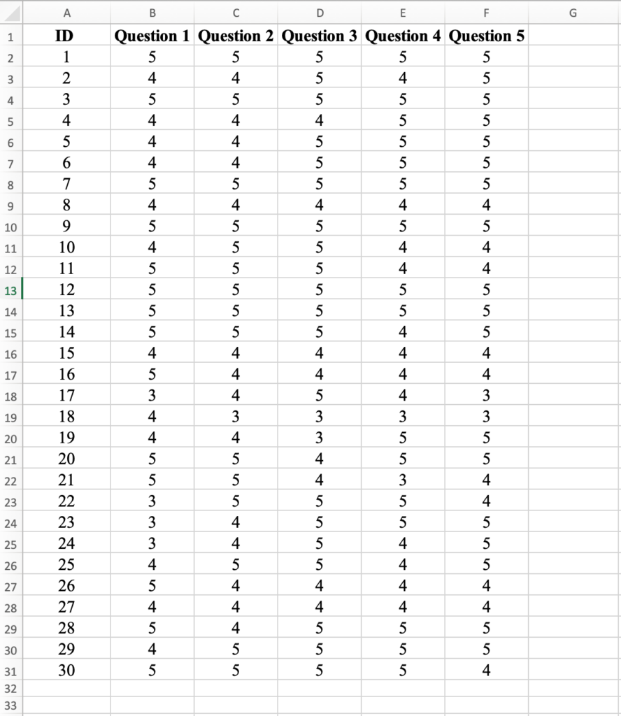 Sample multi-scale questionnaire dataset in Excel.
Step 2: Calculate the Total Score.
Name the column G in the data set Total Score. First, we will have to calculate the Total Score for the first respondent (ID1) by typing =SUM and using the mouse to select the scores for Question 1-5. Close the bracket then press Enter to compute the result.
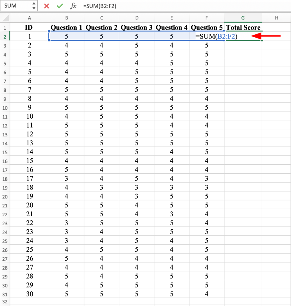 Entering the SUM formula to calculate Total Score for the first respondent.
Next, apply the Total Score formula for ID1 to ID2 to ID30 by dragging it with your mouse to apply it to all respondents.
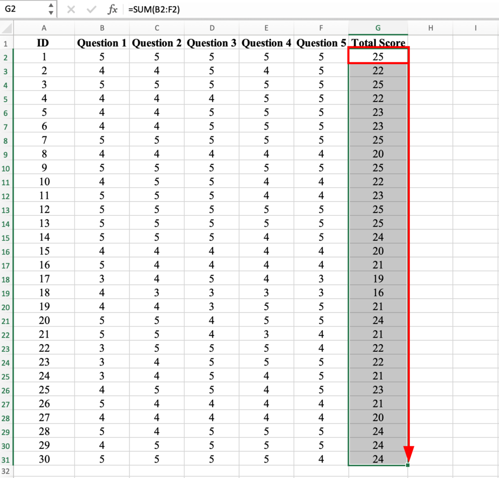 Total Score formula applied to all respondents by dragging down the formula.
Step 3: Calculate the variance for Total Score
Variance measures the degree to which individual scores deviate from the mean score, and it provides information about the spread of scores around the mean.
To calculate variance in Excel, on an empty cell (i.e., column G) type =VAR.S and in the brackets select all the Total Scores values for ID1 to 30. Close the bracket and press the Enter key on your keyboard to compute.
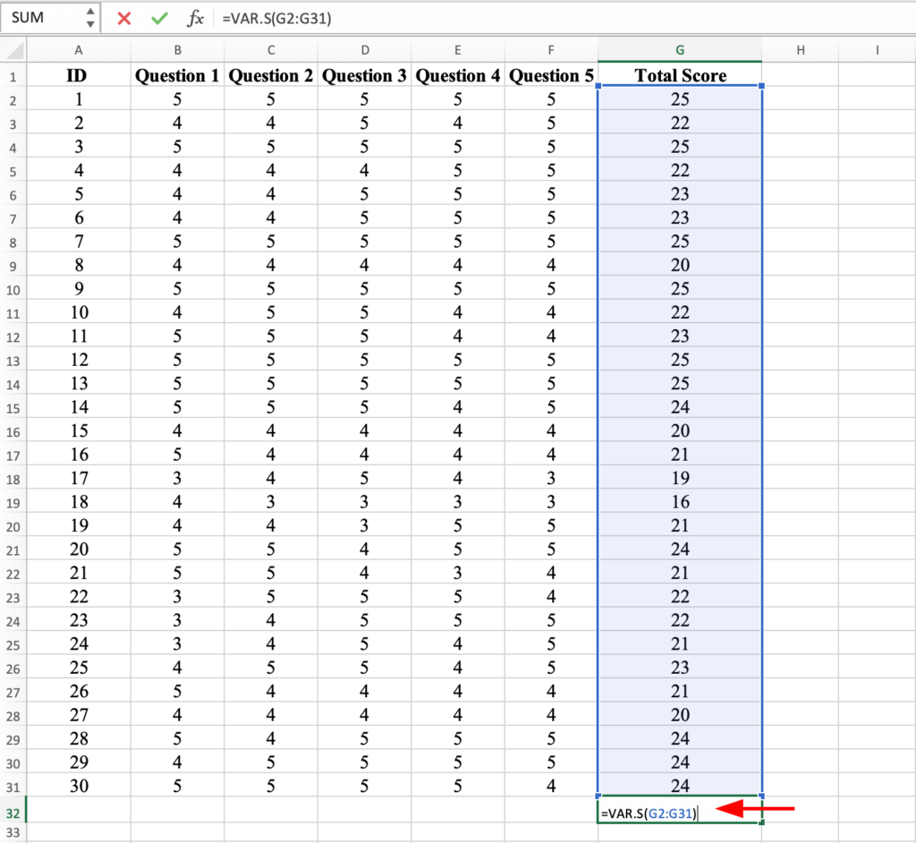 Using VAR.S function to calculate the variance of all Total Scores.
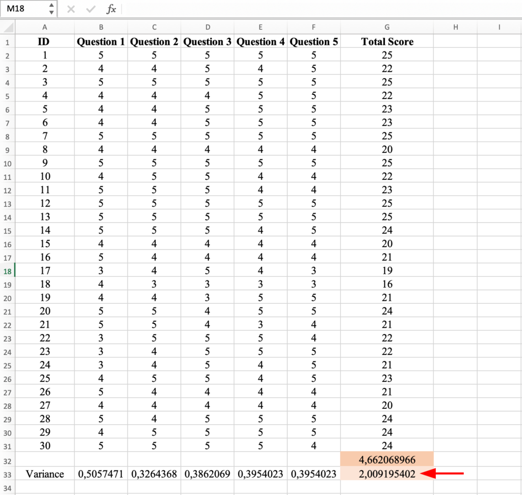
You should get the variance for the Total Score of 4.66 as shown below:
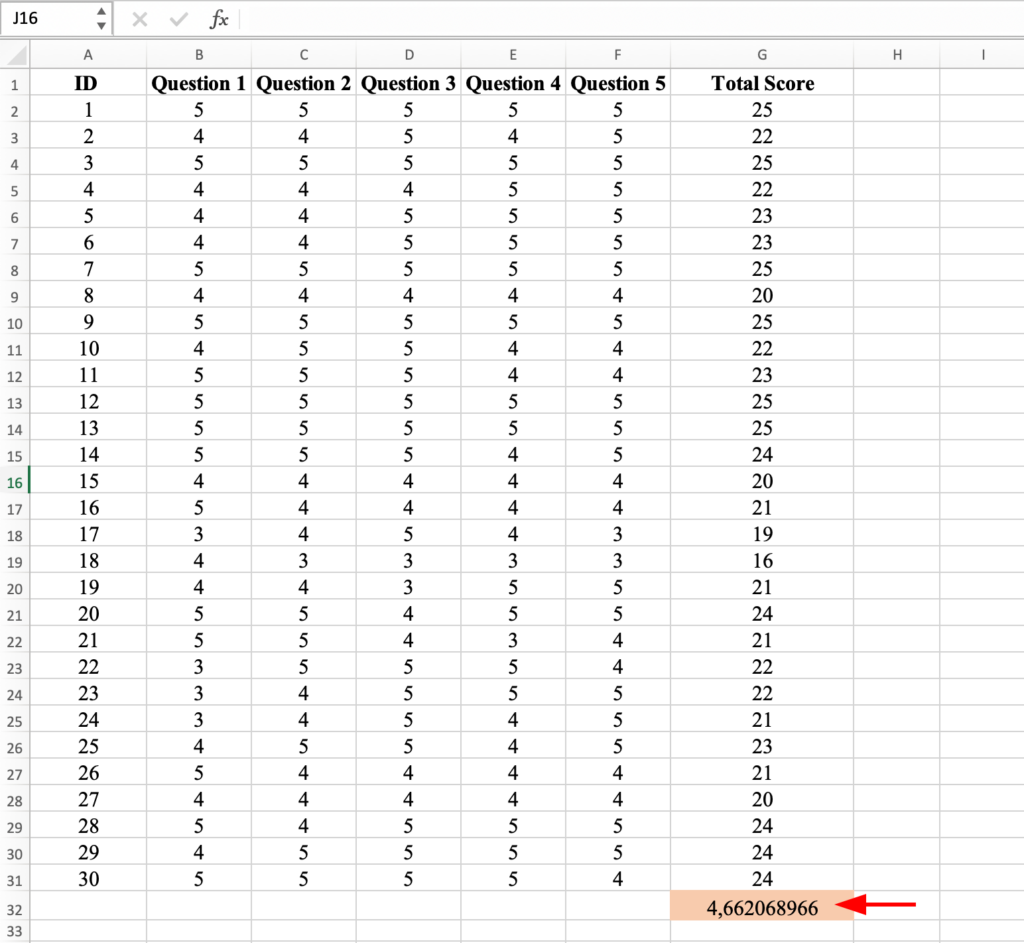 Total Score variance result showing 4.66.
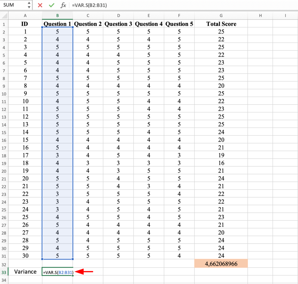
Step 4: Calculate the Variance for all items
Next, let's calculate the variance for the all scores of the Question 1. We will use the same Excel formula for variance =VAR.S and selecting all scores for Question 1. Close the bracket and hit the Enter key.
 Calculating the variance for Question 1 using VAR.S function.
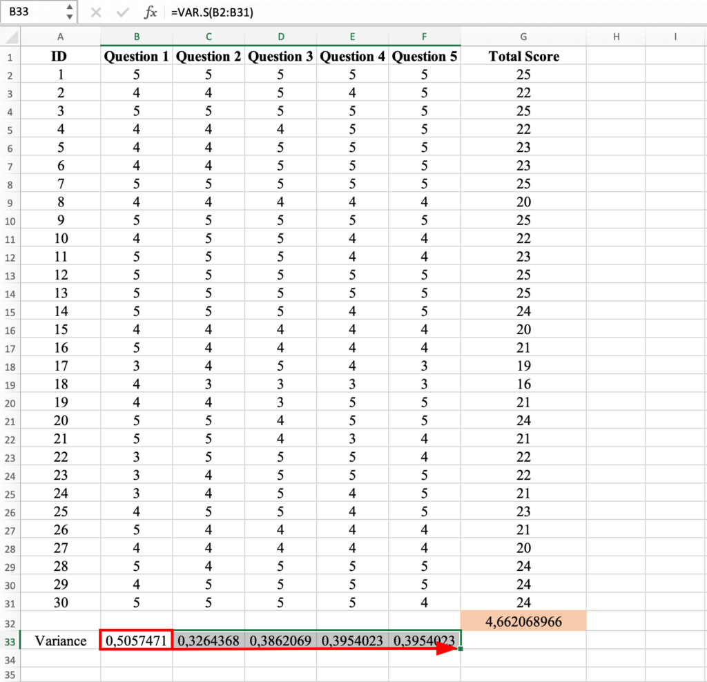
To calculate the variance for the scores in all questions for all respondents, simply apply the variance formula calculated above for the Questions 2-5 as shown below, and press Enter.
 Variance calculated for all items (Questions 1-5) by copying the formula across.
Now we have the variance coefficient for all questions and respondents in our dataset. Well done!
Step 5: Calculate the SUM of Variance for all items
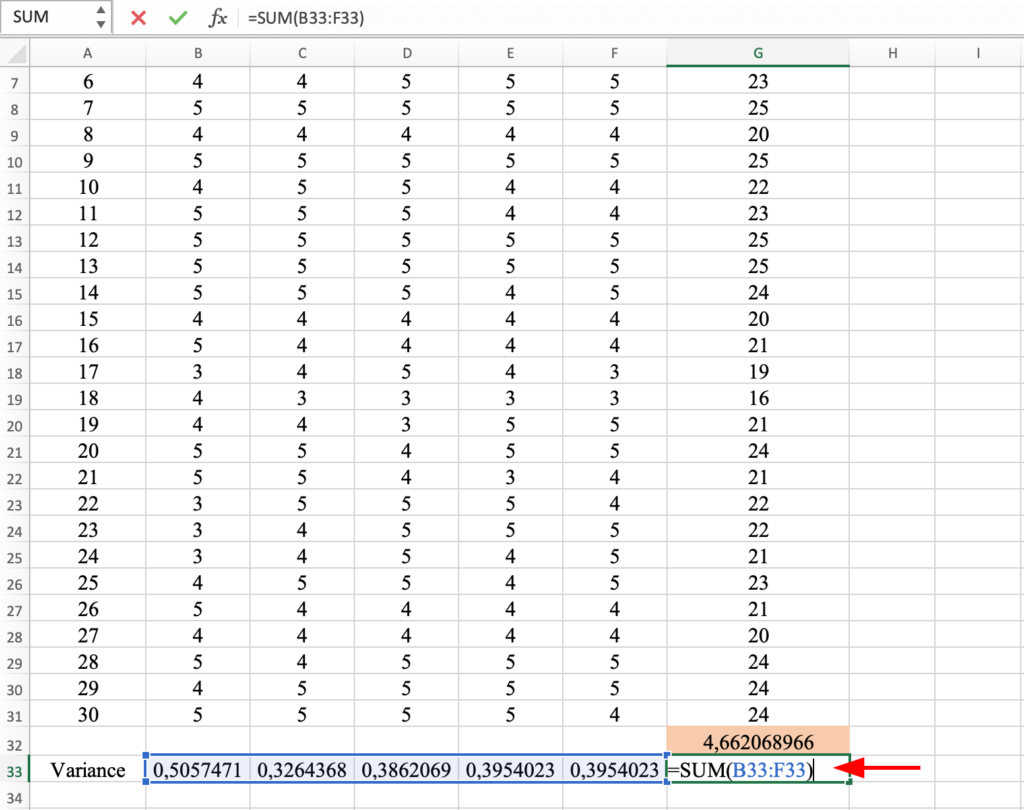
Now we have to calculate the Sum of Variance from the variance calculated above for Questions 1 to 5 using the =SUM formula and selecting the variance coefficient for Question 1-5. Don't forget to close the bracket and hit Enter to compute.
 Using SUM function to calculate the total of all item variances.
The Sum of Variance for all Questions in our dataset is 2.
 Sum of item variances result: 2
Step 6: Calculate Cronbach’s Alpha in Excel
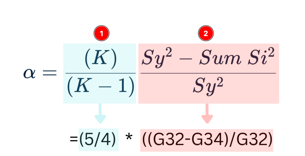
And finally is time to calculate the Alpha coefficient in Excel using the Cronbach's Alpha formula as follows:
-
The first section of the equation is an easy one: we have 5 items (5 questions) in our questionnaire therefore K = 5, divided by K-1 which is 4.
-
The second part of the equation is a bit more complicated, but worry no more, we have everything calculated in Excel already. Sy squared = the variance for the Total Score minus the Sum of Variance for items squared divided by the variance of the Total Score squared.
 Cronbach's Alpha formula entered in Excel with all calculated values.
Sounds complicated, right? Well, you're in luck today. The sheet we used so far in this lesson has Cronbach's Alpha formula for Excel already plugged in.
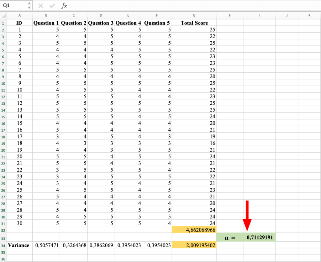 Final Cronbach's Alpha result: 0.71 (Acceptable reliability).
And the Cronbach's Alpha coefficient for our questionnaire is 0.71 therefore the internal consistency is considered acceptable. Mission accomplished.
Frequently Asked Questions
Wrapping Up
In this article we learned how to calculate Cronbach's Alpha in Excel using the Cronbach's Alpha formula, how to interpret reliability coefficient results, and how to fix datasets when alpha values are poor.
Prefer statistical software? Learn how to calculate Cronbach's Alpha in SPSS for one-click reliability testing with item-total statistics.
If you found this Excel reliability calculator guide useful, please share it with your colleagues and friends!
References
Cronbach, L. J. (1951). Coefficient alpha and the internal structure of tests. Psychometrika, 16(3), 297-334.
Nunnally, J. C., & Bernstein, I. H. (1994). Psychometric theory (3rd ed.). New York: McGraw-Hill.