How to test homoscedasticity in R is essential for validating linear regression assumptions. This guide covers two methods: a visual approach using residual plots and the Breusch-Pagan test in R - a statistical test for detecting heteroscedasticity.
Homoscedasticity (constant variance of residuals) is a key assumption in linear regression. When violated, your model's standard errors, confidence intervals, and hypothesis tests become unreliable.
You'll learn how to check homoscedasticity in R using the mtcars dataset, though you can follow along with your own data. Both the visual method and the Breusch-Pagan test will help you determine if your regression model meets the homoscedasticity assumption.
Test Homoscedasticity in R using the Visual Method
The mtcars dataset is built into R, containing information on 32 cars from a 1974 Motor Trend magazine issue. It includes 11 variables such as miles per gallon (mpg), cylinders (cyl), and horsepower (hp).
Create a simple linear regression model using mpg (miles per gallon) as the response variable and hp (horsepower) as the predictor. Use the lm() function:
# Use the mtcars dataset
data(mtcars)

# Create a linear model
model <- lm(mpg ~ hp, data = mtcars)
Use the ggplot2 package to create a scatter plot of residuals against fitted values. Install and load the package:
# Install ggplot2 if not already installed
if (!requireNamespace("ggplot2", quietly = TRUE)) {
 install.packages("ggplot2")
}

# Load ggplot2 package
library(ggplot2)
Create the scatter plot:
# Check for homoscedasticity using residuals vs fitted values plot
residuals_plot <- ggplot(data = mtcars, aes(x = fitted(model), y = resid(model))) +
 geom_point() +
 geom_smooth(method = "loess", se = FALSE, linetype = "dashed") +
 labs(x = "Fitted Values", y = "Residuals") +
 ggtitle("Residuals vs Fitted Values") +
 theme_minimal()

print(residuals_plot)
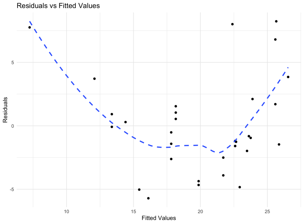 Residuals vs fitted values plot for visual homoscedasticity assessment in R.
Interpretation: In a homoscedastic scenario, residuals should show roughly constant spread across all fitted values. A pattern or funnel shape suggests heteroscedasticity (non-constant variance).
Test Homoscedasticity in R using Breusch-Pagan Test
The Breusch-Pagan test is a statistical method that examines the relationship between squared residuals and fitted values. It provides a formal hypothesis test for homoscedasticity.
Install and load the car package to perform the test:
# Install car package if not already installed
if (!requireNamespace("car", quietly = TRUE)) {
 install.packages("car")
}

# Load car package
library(car)
Perform the Breusch-Pagan test using the ncvTest() function:
# Perform Breusch-Pagan test to check for homoscedasticity
bp_test <- ncvTest(model)
print(bp_test)
Interpreting Breusch-Pagan Test Results
The output includes three key values:
- Chisquare: Test statistic (e.g., 0.0477)
- Df (Degrees of Freedom): Number of parameters tested (typically 1)
- p-value: Probability under the null hypothesis of constant variance (e.g., 0.827)
Interpretation:
- p-value > 0.05: Fail to reject null hypothesis → Assume homoscedasticity (constant variance)
- p-value ≤ 0.05: Reject null hypothesis → Assume heteroscedasticity (non-constant variance)
Example result: Chisquare = 0.0477, Df = 1, p = 0.827
Since p-value (0.827) > 0.05, we fail to reject the null hypothesis and conclude that homoscedasticity is present in the model residuals.
Frequently Asked Questions
Wrapping Up
You now know how to test homoscedasticity in R using two methods: visual residual plots and the Breusch-Pagan test. Both approaches help validate the homoscedasticity assumption in linear regression, ensuring reliable model estimates and hypothesis tests.
Key takeaways:
- Visual method: Check for constant spread in residual plots
- Breusch-Pagan test: Formal statistical test (p > 0.05 = homoscedasticity)
- Violating homoscedasticity leads to unreliable standard errors and confidence intervals
For more on regression assumptions, see our guide on what is homoscedasticity assumption in statistics or learn about moderation analysis in R which also requires homoscedasticity testing.